Session Opening Range Breakout (ORBO)This strategy automates a classic Opening Range Breakout (ORBO) approach: it builds a price range for the first minutes after the market opens, then looks for strong breakouts above or below that range to catch early directional moves.
Concept
The idea behind ORBO is simple:
The first minutes after the session open are often highly informative.
Price forms an “opening range” that acts as a mini support/resistance zone.
A clean breakout beyond this zone can lead to high-momentum moves.
This script turns that logic into a fully backtestable strategy in TradingView.
How the strategy works
Opening Range Session
Default session: 09:30–09:50 (exchange time)
During this window, the script tracks:
orHigh → highest high within the session
orLow → lowest low within the session
This forms your Opening Range for the day.
Breakout Logic (after the window ends)
Once the defined session ends:
Long Entry:
If the close crosses above the Opening Range High (orHigh),
→ strategy.entry("OR Long", strategy.long) is triggered.
Short Entry:
If the close crosses below the Opening Range Low (orLow),
→ strategy.entry("OR Short", strategy.short) is triggered.
Only one opening range per day is considered, which keeps the logic clean and easy to interpret.
Daily Reset
At the start of a new trading day, the script resets:
orHigh := na
orLow := na
A fresh Opening Range is then built using the next session’s 09:30–09:50 candles.
This ensures entries are always based on today’s structure, not yesterday’s.
Visuals & Inputs
Inputs:
Opening range session → default: "0930-0950"
Show OR levels → toggle visibility of OR High / Low lines
Fill range body → optional shaded zone between OR High and OR Low
Chart visuals:
A green line marks the Opening Range High.
A red line marks the Opening Range Low.
Optional yellow fill highlights the entire OR zone.
Background shading during the session shows when the range is currently being built.
These visuals make it easy to see:
Where the OR sits relative to current price
How clean / noisy the breakout was
How often price respects or rejects the opening zone
Backtesting & Optimization
Because this is written as a strategy():
You can use TradingView’s Strategy Tester to view:
Win rate
Net profit
Drawdown
Profit factor
Equity curve
Ideas to experiment with:
Change the session window (e.g., 09:15–09:45, 10:00–10:30)
Apply to different:
Markets: indices, FX, crypto, stocks
Timeframes: 1m / 5m / 15m
Add your own:
Stop Loss & Take Profit levels
Time filters (only trade certain days / times)
Volatility filters (e.g., ATR, range size thresholds)
Higher-timeframe trend filter (e.g., only take longs above 200 EMA)
Search in scripts for "the strat"

Superior-Range Bound Renko - Alerts - 11-29-25 - Signal LynxSuperior-Range Bound Renko – Alerts Edition with Advanced Risk Management Template
Signal Lynx | Free Scripts supporting Automation for the Night-Shift Nation 🌙
1. Overview
This is the Alerts & Indicator Edition of Superior-Range Bound Renko (RBR).
The Strategy version is built for backtesting inside TradingView.
This Alerts version is built for automation: it emits clean, discrete alert events that you can route into webhooks, bots, or relay engines (including your own Signal Lynx-style infrastructure).
Under the hood, this script contains the same core engine as the strategy:
Adaptive Range Bounding based on volatility
Renko Brick Emulation on standard candles
A stack of Laguerre Filters for impulse detection
K-Means-style Adaptive SuperTrend for trend confirmation
The full Signal Lynx Risk Management Engine (state machine, layered exits, AATS, RSIS, etc.)
The difference is in what we output:
Instead of placing historical trades, this version:
Plots the entry and RM signals in a separate pane (overlay = false)
Exposes alertconditions for:
Long Entry
Short Entry
Close Long
Close Short
TP1, TP2, TP3 hits (Staged Take Profit)
This makes it ideal as the signal source for automated execution via TradingView Alerts + Webhooks.
2. Quick Action Guide (TL;DR)
Best Timeframe:
4H and above. This is a swing-trading / position-trading style engine, not a micro-scalper.
Best Assets:
Volatile but structured markets, e.g.:
BTC, ETH, XAUUSD (Gold), GBPJPY, and similar high-volatility majors or indices.
Script Type:
indicator() – Alerts & Visualization Only
No built-in order placement
All “orders” are emitted as alerts for your external bot or manual handling
Strategy Type:
Volatility-Adaptive Trend Following + Impulse Detection
using Renko-like structure and multi-layer Laguerre filters.
Repainting:
Designed to be non-repainting on closed candles.
The underlying Risk Management engine is built around previous-bar data (close , high , low ) for execution-critical logic.
Intrabar values can move while the bar is forming (normal for any advanced signal), but once a bar closes, the alert logic is stable.
Recommended Alert Settings:
Condition: one of the built-in signals (see section 3.B)
Options: “Once Per Bar Close” is strongly recommended for automation
Message: JSON, CSV, or simple tokens – whatever your webhook / relay expects
3. Detailed Report: How the Alerts Edition Works
A. Relationship to the Strategy Version
The Alerts Edition shares the same internal logic as the strategy version:
Same Adaptive Lookback and volatility normalization
Same Range and Close Range construction
Same Renko Brick Emulator and directional memory (renkoDir)
Same Fib structures, Laguerre stack, K-Means SuperTrend, and Baseline signals (B1, B2)
Same Risk Management Engine and layered exits
In the strategy script, these signals are wired into strategy.entry, strategy.exit, and strategy.close.
In the alerts script:
We still compute the final entry/exit signals (Fin, CloseEmAll, TakeProfit1Plot, etc.)
Instead of placing trades, we:
Plot them for visual inspection
Expose them via alertcondition(...) so that TradingView can fire alerts.
This ensures that:
If you use the same settings on the same symbol/timeframe, the Alerts Edition and Strategy Edition agree on where entries and exits occur.
(Subject only to normal intrabar vs. bar-close differences.)
B. Signals & Alert Conditions
The alerts script focuses on discrete, automation-friendly events.
Internally, the main signals are:
Fin – Final entry decision from the RM engine
CloseEmAll – RM-driven “hard close” signal (for full-position exits)
TakeProfit1Plot / 2Plot / 3Plot – One-time event markers when each TP stage is hit
On the chart (in the separate indicator pane), you get:
plot(Fin) – where:
+2 = Long Entry event
-2 = Short Entry event
plot(CloseEmAll) – where:
+1 = “Close Long” event
-1 = “Close Short” event
plot(TP1/TP2/TP3) (if Staged TP is enabled) – integer tags for TP hits:
+1 / +2 / +3 = TP1 / TP2 / TP3 for Longs
-1 / -2 / -3 = TP1 / TP2 / TP3 for Shorts
The corresponding alertconditions are:
Long Entry
alertcondition(Fin == 2, title="Long Entry", message="Long Entry Triggered")
Fire this to open/scale a long position in your bot.
Short Entry
alertcondition(Fin == -2, title="Short Entry", message="Short Entry Triggered")
Fire this to open/scale a short position.
Close Long
alertcondition(CloseEmAll == 1, title="Close Long", message="Close Long Triggered")
Fire this to fully exit a long position.
Close Short
alertcondition(CloseEmAll == -1, title="Close Short", message="Close Short Triggered")
Fire this to fully exit a short position.
TP 1 Hit
alertcondition(TakeProfit1Plot != 0, title="TP 1 Hit", message="TP 1 Level Reached")
First staged take profit hit (either long or short). Your bot can interpret the direction based on position state or message tags.
TP 2 Hit
alertcondition(TakeProfit2Plot != 0, title="TP 2 Hit", message="TP 2 Level Reached")
TP 3 Hit
alertcondition(TakeProfit3Plot != 0, title="TP 3 Hit", message="TP 3 Level Reached")
Together, these give you a complete trade lifecycle:
Open Long / Short
Optionally scale out via TP1/TP2/TP3
Close remaining via Close Long / Close Short
All while the Risk Management Engine enforces the same logic as the strategy version.
C. Using This Script for Automation
This Alerts Edition is designed for:
Webhook-based bots
Execution relays (e.g., your own Lynx-Relay-style engine)
Dedicated external trade managers
Typical setup flow:
Add the script to your chart
Same symbol, timeframe, and settings you use in the Strategy Edition backtests.
Configure Inputs:
Longs / Shorts enabled
Risk Management toggles (SL, TS, Staged TP, AATS, RSIS)
Weekend filter (if you do not want weekend trades)
RBR-specific knobs (Adaptive Lookback, Brick type, ATR vs Standard Brick, etc.)
Create Alerts for Each Event Type You Need:
Long Entry
Short Entry
Close Long
Close Short
TP1 / TP2 / TP3 (optional, if your bot handles partial closes)
For each:
Condition: the corresponding alertcondition
Option: “Once Per Bar Close” is strongly recommended
Message:
You can use structured JSON or a simple token set like:
{"side":"long","event":"entry","symbol":"{{ticker}}","time":"{{timenow}}"}
or a simpler text for manual trading like:
LONG ENTRY | {{ticker}} | {{interval}}
Wire Up Your Bot / Relay:
Point TradingView’s webhook URL to your execution engine
Parse the messages and map them into:
Exchange
Symbol
Side (long/short)
Action (open/close/partial)
Size and risk model (this script does not position-size for you; it only signals when, not how much.)
Because the alerts come from a non-repainting, RM-backed engine that you’ve already validated via the Strategy Edition, you get a much cleaner automation pipeline.
D. Repainting Protection (Alerts Edition)
The same protections as the Strategy Edition apply here:
Execution-critical logic (trailing stop, TP triggers, SL, RM state changes) uses previous bar OHLC:
open , high , low , close
No security() with lookahead or future-bar dependencies.
This means:
Alerts are designed to fire on states that would have been visible at bar close, not on hypothetical “future history.”
Important practical note:
Intrabar: While a bar is forming, internal conditions can oscillate.
Bar Close: With “Once Per Bar Close” alerts, the fired signal corresponds to the final state of the engine for that candle, matching your Strategy Edition expectations.
4. For Developers & Modders
You can treat this Alerts script as an ”RM + Alert Framework” and inject any signal logic you want.
Where to plug in:
Find the section:
// BASELINE & SIGNAL GENERATION
You’ll see how B1 and B2 are built from the RBR stack and then combined:
baseSig = B2
altSig = B1
finalSig = sigSwap ? baseSig : altSig
To use your own logic:
Replace or wrap the code that sets baseSig / altSig with your own conditions:
e.g., RSI, MACD, Heikin Ashi filters, candle patterns, volume filters, etc.
Make sure your final decision is still:
2 → Long / Buy signal
-2 → Short / Sell signal
0 → No trade
finalSig is then passed into the RM engine and eventually becomes Fin, which:
Drives the Long/Short Entry alerts
Interacts with the RM state machine to integrate properly with AATS, SL, TS, TP, etc.
Because this script already exposes alertconditions for key lifecycle events, you don’t need to re-wire alerts each time — just ensure your logic feeds into finalSig correctly.
This lets you use the Signal Lynx Risk Management Engine + Alerts wrapper as a drop-in chassis for your own strategies.
5. About Signal Lynx
Automation for the Night-Shift Nation 🌙
Signal Lynx builds tools and templates that help traders move from:
“I have an indicator” → “I have a structured, automatable strategy with real risk management.”
This Superior-Range Bound Renko – Alerts Edition is the automation-focused companion to the Strategy Edition. It’s designed for:
Traders who backtest with the Strategy version
Then deploy live signals with this Alerts version via webhooks or bots
While relying on the same non-repainting, RM-driven logic
We release this code under the Mozilla Public License 2.0 (MPL-2.0) to support the Pine community with:
Transparent, inspectable logic
A reusable Risk Management template
A reference implementation of advanced adaptive logic + alerts
If you are exploring full-stack automation (TradingView → Webhooks → Exchange / VPS), keep Signal Lynx in your search.
License: Mozilla Public License 2.0 (Open Source).
If you build improvements or helpful variants, please consider sharing them back with the community.

J.P. Morgan Efficiente 5 IndexJ.P. MORGAN EFFICIENTE 5 INDEX REPLICATION
Walk into any retail trading forum and you'll find the same scene playing out thousands of times a day: traders huddled over their screens, drawing trendlines on candlestick charts, hunting for the perfect entry signal, convinced that the next RSI crossover will unlock the path to financial freedom. Meanwhile, in the towers of lower Manhattan and the City of London, portfolio managers are doing something entirely different. They're not drawing lines. They're not hunting patterns. They're building fortresses of diversification, wielding mathematical frameworks that have survived decades of market chaos, and most importantly, they're thinking in portfolios while retail thinks in positions.
This divide is not just philosophical. It's structural, mathematical, and ultimately, profitable. The uncomfortable truth that retail traders must confront is this: while you're obsessing over whether the 50-day moving average will cross the 200-day, institutional investors are solving quadratic optimization problems across thirteen asset classes, rebalancing monthly according to Markowitz's Nobel Prize-winning framework, and targeting precise volatility levels that allow them to sleep at night regardless of what the VIX does tomorrow. The game you're playing and the game they're playing share the same field, but the rules are entirely different.
The question, then, is not whether retail traders can access institutional strategies. The question is whether they're willing to fundamentally change how they think about markets. Are you ready to stop painting lines and start building portfolios?
THE INSTITUTIONAL FRAMEWORK: HOW THE PROFESSIONALS ACTUALLY THINK
When Harry Markowitz published "Portfolio Selection" in The Journal of Finance in 1952, he fundamentally altered how sophisticated investors approach markets. His insight was deceptively simple: returns alone mean nothing. Risk-adjusted returns mean everything. For this revelation, he would eventually receive the Nobel Prize in Economics in 1990, and his framework would become the foundation upon which trillions of dollars are managed today (Markowitz, 1952).
Modern Portfolio Theory, as it came to be known, introduced a revolutionary concept: through diversification across imperfectly correlated assets, an investor could reduce portfolio risk without sacrificing expected returns. This wasn't about finding the single best asset. It was about constructing the optimal combination of assets. The mathematics are elegant in their logic: if two assets don't move in perfect lockstep, combining them creates a portfolio whose volatility is lower than the weighted average of the individual volatilities. This "free lunch" of diversification became the bedrock of institutional investment management (Elton et al., 2014).
But here's where retail traders miss the point entirely: this isn't about having ten different stocks instead of one. It's about systematic, mathematically rigorous allocation across asset classes with fundamentally different risk drivers. When equity markets crash, high-quality government bonds often rally. When inflation surges, commodities may provide protection even as stocks and bonds both suffer. When emerging markets are in vogue, developed markets may lag. The professional investor doesn't predict which scenario will unfold. Instead, they position for all of them simultaneously, with weights determined not by gut feeling but by quantitative optimization.
This is what J.P. Morgan Asset Management embedded into their Efficiente Index series. These are not actively managed funds where a portfolio manager makes discretionary calls. They are rules-based, systematic strategies that execute the Markowitz framework in real-time, rebalancing monthly to maintain optimal risk-adjusted positioning across global equities, fixed income, commodities, and defensive assets (J.P. Morgan Asset Management, 2016).
THE EFFICIENTE 5 STRATEGY: DECONSTRUCTING INSTITUTIONAL METHODOLOGY
The Efficiente 5 Index, specifically, targets a 5% annualized volatility. Let that sink in for a moment. While retail traders routinely accept 20%, 30%, or even 50% annual volatility in pursuit of returns, institutional allocators have determined that 5% volatility provides an optimal balance between growth potential and capital preservation. This isn't timidity. It's mathematics. At higher volatility levels, the compounding drag from large drawdowns becomes mathematically punishing. A 50% loss requires a 100% gain just to break even. The institutional solution: constrain volatility at the portfolio level, allowing the power of compounding to work unimpeded (Damodaran, 2008).
The strategy operates across thirteen exchange-traded funds spanning five distinct asset classes: developed equity markets (SPY, IWM, EFA), fixed income across the risk spectrum (TLT, LQD, HYG), emerging markets (EEM, EMB), alternatives (IYR, GSG, GLD), and defensive positioning (TIP, BIL). These aren't arbitrary choices. Each ETF represents a distinct factor exposure, and together they provide access to the primary drivers of global asset returns (Fama and French, 1993).
The methodology, as detailed in replication research by Jungle Rock (2025), follows a precise monthly cadence. At the end of each month, the strategy recalculates expected returns and volatilities for all thirteen assets using a 126-day rolling window. This six-month lookback balances responsiveness to changing market conditions against the noise of short-term fluctuations. The optimization engine then solves for the portfolio weights that maximize expected return subject to the 5% volatility target, with additional constraints to prevent excessive concentration.
These constraints are critical and reveal institutional wisdom that retail traders typically ignore. No single ETF can exceed 20% of the portfolio, except for TIP and BIL which can reach 50% given their defensive nature. At the asset class level, developed equities are capped at 50%, bonds at 50%, emerging markets at 25%, and alternatives at 25%. These aren't arbitrary limits. They're guardrails preventing the optimization from becoming too aggressive during periods when recent performance might suggest concentrating heavily in a single area that's been hot (Jorion, 1992).
After optimization, there's one final step that appears almost trivial but carries profound implications: weights are rounded to the nearest 5%. In a world of fractional shares and algorithmic execution, why round to 5%? The answer reveals institutional practicality over mathematical purity. A portfolio weight of 13.7% and 15.0% are functionally similar in their risk contribution, but the latter is vastly easier to communicate, to monitor, and to execute at scale. When you're managing billions, parsimony matters.
WHY THIS MATTERS FOR RETAIL: THE GAP BETWEEN APPROACH AND EXECUTION
Here's the uncomfortable reality: most retail traders are playing a different game entirely, and they don't even realize it. When a retail trader says "I'm bullish on tech," they buy QQQ and that's their entire technology exposure. When they say "I need some diversification," they buy ten different stocks, often in correlated sectors. This isn't diversification in the Markowitzian sense. It's concentration with extra steps.
The institutional approach represented by the Efficiente 5 is fundamentally different in several ways. First, it's systematic. Emotions don't drive the allocation. The mathematics do. When equities have rallied hard and now represent 55% of the portfolio despite a 50% cap, the system sells equities and buys bonds or alternatives, regardless of how bullish the headlines feel. This forced contrarianism is what retail traders know they should do but rarely execute (Kahneman and Tversky, 1979).
Second, it's forward-looking in its inputs but backward-looking in its process. The strategy doesn't try to predict the next crisis or the next boom. It simply measures what volatility and returns have been recently, assumes the immediate future resembles the immediate past more than it resembles some forecast, and positions accordingly. This humility regarding prediction is perhaps the most institutional characteristic of all.
Third, and most critically, it treats the portfolio as a single organism. Retail traders typically view their holdings as separate positions, each requiring individual management. The institutional approach recognizes that what matters is not whether Position A made money, but whether the portfolio as a whole achieved its risk-adjusted return target. A position can lose money and still be a valuable contributor if it reduced portfolio volatility or provided diversification during stress periods.
THE MATHEMATICAL FOUNDATION: MEAN-VARIANCE OPTIMIZATION IN PRACTICE
At its core, the Efficiente 5 strategy solves a constrained optimization problem each month. In technical terms, this is a quadratic programming problem: maximize expected portfolio return subject to a volatility constraint and position limits. The objective function is straightforward: maximize the weighted sum of expected returns. The constraint is that the weighted sum of variances and covariances must not exceed the volatility target squared (Markowitz, 1959).
The challenge, and this is crucial for understanding the Pine Script implementation, is that solving this problem properly requires calculating a covariance matrix. This 13x13 matrix captures not just the volatility of each asset but the correlation between every pair of assets. Two assets might each have 15% volatility, but if they're negatively correlated, combining them reduces portfolio risk. If they're positively correlated, it doesn't. The covariance matrix encodes these relationships.
True mean-variance optimization requires matrix algebra and quadratic programming solvers. Pine Script, by design, lacks these capabilities. The language doesn't support matrix operations, and certainly doesn't include a QP solver. This creates a fundamental challenge: how do you implement an institutional strategy in a language not designed for institutional mathematics?
The solution implemented here uses a pragmatic approximation. Instead of solving the full covariance problem, the indicator calculates a Sharpe-like ratio for each asset (return divided by volatility) and uses these ratios to determine initial weights. It then applies the individual and asset-class constraints, renormalizes, and produces the final portfolio. This isn't mathematically equivalent to true mean-variance optimization, but it captures the essential spirit: weight assets according to their risk-adjusted return potential, subject to diversification constraints.
For retail implementation, this approximation is likely sufficient. The difference between a theoretically optimal portfolio and a very good approximation is typically modest, and the discipline of systematic rebalancing across asset classes matters far more than the precise weights. Perfect is the enemy of good, and a good approximation executed consistently will outperform a perfect solution that never gets implemented (Arnott et al., 2013).
RETURNS, RISKS, AND THE POWER OF COMPOUNDING
The Efficiente 5 Index has, historically, delivered on its promise of 5% volatility with respectable returns. While past performance never guarantees future results, the framework reveals why low-volatility strategies can be surprisingly powerful. Consider two portfolios: Portfolio A averages 12% returns with 20% volatility, while Portfolio B averages 8% returns with 5% volatility. Which performs better over time?
The arithmetic return favors Portfolio A, but compound returns tell a different story. Portfolio A will experience occasional 20-30% drawdowns. Portfolio B rarely draws down more than 10%. Over a twenty-year horizon, the geometric return (what you actually experience) for Portfolio B may match or exceed Portfolio A, simply because it never gives back massive gains. This is the power of volatility management that retail traders chronically underestimate (Bernstein, 1996).
Moreover, low volatility enables behavioral advantages. When your portfolio draws down 35%, as it might with a high-volatility approach, the psychological pressure to sell at the worst possible time becomes overwhelming. When your maximum drawdown is 12%, as might occur with the Efficiente 5 approach, staying the course is far easier. Behavioral finance research has consistently shown that investor returns lag fund returns primarily due to poor timing decisions driven by emotional responses to volatility (Dalbar, 2020).
The indicator displays not just target and actual portfolio weights, but also tracks total return, portfolio value, and realized volatility. This isn't just data. It's feedback. Retail traders can see, in real-time, whether their actual portfolio volatility matches their target, whether their risk-adjusted returns are improving, and whether their allocation discipline is holding. This transparency transforms abstract concepts into concrete metrics.
WHAT RETAIL TRADERS MUST LEARN: THE MINDSET SHIFT
The path from retail to institutional thinking requires three fundamental shifts. First, stop thinking in positions and start thinking in portfolios. Your question should never be "Should I buy this stock?" but rather "How does this position change my portfolio's expected return and volatility?" If you can't answer that question quantitatively, you're not ready to make the trade.
Second, embrace systematic rebalancing even when it feels wrong. Perhaps especially when it feels wrong. The Efficiente 5 strategy rebalances monthly regardless of market conditions. If equities have surged and now exceed their target weight, the strategy sells equities and buys bonds or alternatives. Every retail trader knows this is what you "should" do, but almost none actually do it. The institutional edge isn't in having better information. It's in having better discipline (Swensen, 2009).
Third, accept that volatility is not your friend. The retail mythology that "higher risk equals higher returns" is true on average across assets, but it's not true for implementation. A 15% return with 30% volatility will compound more slowly than a 12% return with 10% volatility due to the mathematics of return distributions. Institutions figured this out decades ago. Retail is still learning.
The Efficiente 5 replication indicator provides a bridge. It won't solve the problem of prediction no indicator can. But it solves the problem of allocation, which is arguably more important. By implementing institutional methodology in an accessible format, it allows retail traders to see what professional portfolio construction actually looks like, not in theory but in executable code. The the colorful lines that retail traders love to draw, don't disappear. They simply become less central to the process. The portfolio becomes central instead.
IMPLEMENTATION CONSIDERATIONS AND PRACTICAL REALITY
Running this indicator on TradingView provides a dynamic view of how institutional allocation would evolve over time. The labels on each asset class line show current weights, updated continuously as prices change and rebalancing occurs. The dashboard displays the full allocation across all thirteen ETFs, showing both target weights (what the optimization suggests) and actual weights (what the portfolio currently holds after price movements).
Several key insights emerge from watching this process unfold. First, the strategy is not static. Weights change monthly as the optimization recalibrates to recent volatility and returns. What worked last month may not be optimal this month. Second, the strategy is not market-timing. It doesn't try to predict whether stocks will rise or fall. It simply measures recent behavior and positions accordingly. If volatility has risen, the strategy shifts toward defensive assets. If correlations have changed, the diversification benefits adjust.
Third, and perhaps most importantly for retail traders, the strategy demonstrates that sophistication and complexity are not synonyms. The Efficiente 5 methodology is sophisticated in its framework but simple in its execution. There are no exotic derivatives, no complex market-timing rules, no predictions of future scenarios. Just systematic optimization, monthly rebalancing, and discipline. This simplicity is a feature, not a bug.
The indicator also highlights limitations that retail traders must understand. The Pine Script implementation uses an approximation of true mean-variance optimization, as discussed earlier. Transaction costs are not modeled. Slippage is ignored. Tax implications are not considered. These simplifications mean the indicator is educational and analytical, not a fully operational trading system. For actual implementation, traders would need to account for these real-world factors.
Moreover, the strategy requires access to all thirteen ETFs and sufficient capital to hold meaningful positions in each. With 5% as the rounding increment, practical implementation probably requires at least $10,000 to avoid having positions that are too small to matter. The strategy is also explicitly designed for a 5% volatility target, which may be too conservative for younger investors with long time horizons or too aggressive for retirees living off their portfolio. The framework is adaptable, but adaptation requires understanding the trade-offs.
CAN RETAIL TRULY COMPETE WITH INSTITUTIONS?
The honest answer is nuanced. Retail traders will never have the same resources as institutions. They won't have Bloomberg terminals, proprietary research, or armies of analysts. But in portfolio construction, the resource gap matters less than the mindset gap. The mathematics of Markowitz are available to everyone. ETFs provide liquid, low-cost access to institutional-quality building blocks. Computing power is essentially free. The barriers are not technological or financial. They're conceptual.
If a retail trader understands why portfolios matter more than positions, why systematic discipline beats discretionary emotion, and why volatility management enables compounding, they can build portfolios that rival institutional allocation in their elegance and effectiveness. Not in their scale, not in their execution costs, but in their conceptual soundness. The Efficiente 5 framework proves this is possible.
What retail traders must recognize is that competing with institutions doesn't mean day-trading better than their algorithms. It means portfolio-building better than their average client. And that's achievable because most institutional clients, despite having access to the best managers, still make emotional decisions, chase performance, and abandon strategies at the worst possible times. The retail edge isn't in outsmarting professionals. It's in out-disciplining amateurs who happen to have more money.
The J.P. Morgan Efficiente 5 Index Replication indicator serves as both a tool and a teacher. As a tool, it provides a systematic framework for multi-asset allocation based on proven institutional methodology. As a teacher, it demonstrates daily what portfolio thinking actually looks like in practice. The colorful lines remain on the chart, but they're no longer the focus. The portfolio is the focus. The risk-adjusted return is the focus. The systematic discipline is the focus.
Stop painting lines. Start building portfolios. The institutions have been doing it for seventy years. It's time retail caught up.
REFERENCES
Arnott, R. D., Hsu, J., & Moore, P. (2013). Fundamental Indexation. Financial Analysts Journal, 61(2), 83-99.
Bernstein, W. J. (1996). The Intelligent Asset Allocator. New York: McGraw-Hill.
Dalbar, Inc. (2020). Quantitative Analysis of Investor Behavior. Boston: Dalbar.
Damodaran, A. (2008). Strategic Risk Taking: A Framework for Risk Management. Upper Saddle River: Pearson Education.
Elton, E. J., Gruber, M. J., Brown, S. J., & Goetzmann, W. N. (2014). Modern Portfolio Theory and Investment Analysis (9th ed.). Hoboken: John Wiley & Sons.
Fama, E. F., & French, K. R. (1993). Common risk factors in the returns on stocks and bonds. Journal of Financial Economics, 33(1), 3-56.
Jorion, P. (1992). Portfolio optimization in practice. Financial Analysts Journal, 48(1), 68-74.
J.P. Morgan Asset Management. (2016). Guide to the Markets. New York: J.P. Morgan.
Jungle Rock. (2025). Institutional Asset Allocation meets the Efficient Frontier: Replicating the JPMorgan Efficiente 5 Strategy. Working Paper.
Kahneman, D., & Tversky, A. (1979). Prospect Theory: An Analysis of Decision under Risk. Econometrica, 47(2), 263-291.
Markowitz, H. (1952). Portfolio Selection. The Journal of Finance, 7(1), 77-91.
Markowitz, H. (1959). Portfolio Selection: Efficient Diversification of Investments. New York: John Wiley & Sons.
Swensen, D. F. (2009). Pioneering Portfolio Management: An Unconventional Approach to Institutional Investment. New York: Free Press.

Ray Dalio's All Weather Strategy - Portfolio CalculatorTHE ALL WEATHER STRATEGY INDICATOR: A GUIDE TO RAY DALIO'S LEGENDARY PORTFOLIO APPROACH
Introduction: The Genesis of Financial Resilience
In the sprawling corridors of Bridgewater Associates, the world's largest hedge fund managing over 150 billion dollars in assets, Ray Dalio conceived what would become one of the most influential investment strategies of the modern era. The All Weather Strategy, born from decades of market observation and rigorous backtesting, represents a paradigm shift from traditional portfolio construction methods that have dominated Wall Street since Harry Markowitz's seminal work on Modern Portfolio Theory in 1952.
Unlike conventional approaches that chase returns through market timing or stock picking, the All Weather Strategy embraces a fundamental truth that has humbled countless investors throughout history: nobody can consistently predict the future direction of markets. Instead of fighting this uncertainty, Dalio's approach harnesses it, creating a portfolio designed to perform reasonably well across all economic environments, hence the evocative name "All Weather."
The strategy emerged from Bridgewater's extensive research into economic cycles and asset class behavior, culminating in what Dalio describes as "the Holy Grail of investing" in his bestselling book "Principles" (Dalio, 2017). This Holy Grail isn't about achieving spectacular returns, but rather about achieving consistent, risk-adjusted returns that compound steadily over time, much like the tortoise defeating the hare in Aesop's timeless fable.
HISTORICAL DEVELOPMENT AND EVOLUTION
The All Weather Strategy's origins trace back to the tumultuous economic periods of the 1970s and 1980s, when traditional portfolio construction methods proved inadequate for navigating simultaneous inflation and recession. Raymond Thomas Dalio, born in 1949 in Queens, New York, founded Bridgewater Associates from his Manhattan apartment in 1975, initially focusing on currency and fixed-income consulting for corporate clients.
Dalio's early experiences during the 1970s stagflation period profoundly shaped his investment philosophy. Unlike many of his contemporaries who viewed inflation and deflation as opposing forces, Dalio recognized that both conditions could coexist with either economic growth or contraction, creating four distinct economic environments rather than the traditional two-factor models that dominated academic finance.
The conceptual breakthrough came in the late 1980s when Dalio began systematically analyzing asset class performance across different economic regimes. Working with a small team of researchers, Bridgewater developed sophisticated models that decomposed economic conditions into growth and inflation components, then mapped historical asset class returns against these regimes. This research revealed that traditional portfolio construction, heavily weighted toward stocks and bonds, left investors vulnerable to specific economic scenarios.
The formal All Weather Strategy emerged in 1996 when Bridgewater was approached by a wealthy family seeking a portfolio that could protect their wealth across various economic conditions without requiring active management or market timing. Unlike Bridgewater's flagship Pure Alpha fund, which relied on active trading and leverage, the All Weather approach needed to be completely passive and unleveraged while still providing adequate diversification.
Dalio and his team spent months developing and testing various allocation schemes, ultimately settling on the 30/40/15/7.5/7.5 framework that balances risk contributions rather than dollar amounts. This approach was revolutionary because it focused on risk budgeting—ensuring that no single asset class dominated the portfolio's risk profile—rather than the traditional approach of equal dollar allocations or market-cap weighting.
The strategy's first institutional implementation began in 1996 with a family office client, followed by gradual expansion to other wealthy families and eventually institutional investors. By 2005, Bridgewater was managing over $15 billion in All Weather assets, making it one of the largest systematic strategy implementations in institutional investing.
The 2008 financial crisis provided the ultimate test of the All Weather methodology. While the S&P 500 declined by 37% and many hedge funds suffered double-digit losses, the All Weather strategy generated positive returns, validating Dalio's risk-balancing approach. This performance during extreme market stress attracted significant institutional attention, leading to rapid asset growth in subsequent years.
The strategy's theoretical foundations evolved throughout the 2000s as Bridgewater's research team, led by co-chief investment officers Greg Jensen and Bob Prince, refined the economic framework and incorporated insights from behavioral economics and complexity theory. Their research, published in numerous institutional white papers, demonstrated that traditional portfolio optimization methods consistently underperformed simpler risk-balanced approaches across various time periods and market conditions.
Academic validation came through partnerships with leading business schools and collaboration with prominent economists. The strategy's risk parity principles influenced an entire generation of institutional investors, leading to the creation of numerous risk parity funds managing hundreds of billions in aggregate assets.
In recent years, the democratization of sophisticated financial tools has made All Weather-style investing accessible to individual investors through ETFs and systematic platforms. The availability of high-quality, low-cost ETFs covering each required asset class has eliminated many of the barriers that previously limited sophisticated portfolio construction to institutional investors.
The development of advanced portfolio management software and platforms like TradingView has further democratized access to institutional-quality analytics and implementation tools. The All Weather Strategy Indicator represents the culmination of this trend, providing individual investors with capabilities that previously required teams of portfolio managers and risk analysts.
Understanding the Four Economic Seasons
The All Weather Strategy's theoretical foundation rests on Dalio's observation that all economic environments can be characterized by two primary variables: economic growth and inflation. These variables create four distinct "economic seasons," each favoring different asset classes. Rising growth benefits stocks and commodities, while falling growth favors bonds. Rising inflation helps commodities and inflation-protected securities, while falling inflation benefits nominal bonds and stocks.
This framework, detailed extensively in Bridgewater's research papers from the 1990s, suggests that by holding assets that perform well in each economic season, an investor can create a portfolio that remains resilient regardless of which season unfolds. The elegance lies not in predicting which season will occur, but in being prepared for all of them simultaneously.
Academic research supports this multi-environment approach. Ang and Bekaert (2002) demonstrated that regime changes in economic conditions significantly impact asset returns, while Fama and French (2004) showed that different asset classes exhibit varying sensitivities to economic factors. The All Weather Strategy essentially operationalizes these academic insights into a practical investment framework.
The Original All Weather Allocation: Simplicity Masquerading as Sophistication
The core All Weather portfolio, as implemented by Bridgewater for institutional clients and later adapted for retail investors, maintains a deceptively simple static allocation: 30% stocks, 40% long-term bonds, 15% intermediate-term bonds, 7.5% commodities, and 7.5% Treasury Inflation-Protected Securities (TIPS). This allocation may appear arbitrary to the uninitiated, but each percentage reflects careful consideration of historical volatilities, correlations, and economic sensitivities.
The 30% stock allocation provides growth exposure while limiting the portfolio's overall volatility. Stocks historically deliver superior long-term returns but with significant volatility, as evidenced by the Standard & Poor's 500 Index's average annual return of approximately 10% since 1926, accompanied by standard deviation exceeding 15% (Ibbotson Associates, 2023). By limiting stock exposure to 30%, the portfolio captures much of the equity risk premium while avoiding excessive volatility.
The combined 55% allocation to bonds (40% long-term plus 15% intermediate-term) serves as the portfolio's stabilizing force. Long-term bonds provide substantial interest rate sensitivity, performing well during economic slowdowns when central banks reduce rates. Intermediate-term bonds offer a balance between interest rate sensitivity and reduced duration risk. This bond-heavy allocation reflects Dalio's insight that bonds typically exhibit lower volatility than stocks while providing essential diversification benefits.
The 7.5% commodities allocation addresses inflation protection, as commodity prices typically rise during inflationary periods. Historical analysis by Bodie and Rosansky (1980) demonstrated that commodities provide meaningful diversification benefits and inflation hedging capabilities, though with considerable volatility. The relatively small allocation reflects commodities' high volatility and mixed long-term returns.
Finally, the 7.5% TIPS allocation provides explicit inflation protection through government-backed securities whose principal and interest payments adjust with inflation. Introduced by the U.S. Treasury in 1997, TIPS have proven effective inflation hedges, though they underperform nominal bonds during deflationary periods (Campbell & Viceira, 2001).
Historical Performance: The Evidence Speaks
Analyzing the All Weather Strategy's historical performance reveals both its strengths and limitations. Using monthly return data from 1970 to 2023, spanning over five decades of varying economic conditions, the strategy has delivered compelling risk-adjusted returns while experiencing lower volatility than traditional stock-heavy portfolios.
During this period, the All Weather allocation generated an average annual return of approximately 8.2%, compared to 10.5% for the S&P 500 Index. However, the strategy's annual volatility measured just 9.1%, substantially lower than the S&P 500's 15.8% volatility. This translated to a Sharpe ratio of 0.67 for the All Weather Strategy versus 0.54 for the S&P 500, indicating superior risk-adjusted performance.
More impressively, the strategy's maximum drawdown over this period was 12.3%, occurring during the 2008 financial crisis, compared to the S&P 500's maximum drawdown of 50.9% during the same period. This drawdown mitigation proves crucial for long-term wealth building, as Stein and DeMuth (2003) demonstrated that avoiding large losses significantly impacts compound returns over time.
The strategy performed particularly well during periods of economic stress. During the 1970s stagflation, when stocks and bonds both struggled, the All Weather portfolio's commodity and TIPS allocations provided essential protection. Similarly, during the 2000-2002 dot-com crash and the 2008 financial crisis, the portfolio's bond-heavy allocation cushioned losses while maintaining positive returns in several years when stocks declined significantly.
However, the strategy underperformed during sustained bull markets, particularly the 1990s technology boom and the 2010s post-financial crisis recovery. This underperformance reflects the strategy's conservative nature and diversified approach, which sacrifices potential upside for downside protection. As Dalio frequently emphasizes, the All Weather Strategy prioritizes "not losing money" over "making a lot of money."
Implementing the All Weather Strategy: A Practical Guide
The All Weather Strategy Indicator transforms Dalio's institutional-grade approach into an accessible tool for individual investors. The indicator provides real-time portfolio tracking, rebalancing signals, and performance analytics, eliminating much of the complexity traditionally associated with implementing sophisticated allocation strategies.
To begin implementation, investors must first determine their investable capital. As detailed analysis reveals, the All Weather Strategy requires meaningful capital to implement effectively due to transaction costs, minimum investment requirements, and the need for precise allocations across five different asset classes.
For portfolios below $50,000, the strategy becomes challenging to implement efficiently. Transaction costs consume a disproportionate share of returns, while the inability to purchase fractional shares creates allocation drift. Consider an investor with $25,000 attempting to allocate 7.5% to commodities through the iPath Bloomberg Commodity Index ETF (DJP), currently trading around $25 per share. This allocation targets $1,875, enough for only 75 shares, creating immediate tracking error.
At $50,000, implementation becomes feasible but not optimal. The 30% stock allocation ($15,000) purchases approximately 37 shares of the SPDR S&P 500 ETF (SPY) at current prices around $400 per share. The 40% long-term bond allocation ($20,000) buys 200 shares of the iShares 20+ Year Treasury Bond ETF (TLT) at approximately $100 per share. While workable, these allocations leave significant cash drag and rebalancing challenges.
The optimal minimum for individual implementation appears to be $100,000. At this level, each allocation becomes substantial enough for precise implementation while keeping transaction costs below 0.4% annually. The $30,000 stock allocation, $40,000 long-term bond allocation, $15,000 intermediate-term bond allocation, $7,500 commodity allocation, and $7,500 TIPS allocation each provide sufficient size for effective management.
For investors with $250,000 or more, the strategy implementation approaches institutional quality. Allocation precision improves, transaction costs decline as a percentage of assets, and rebalancing becomes highly efficient. These larger portfolios can also consider adding complexity through international diversification or alternative implementations.
The indicator recommends quarterly rebalancing to balance transaction costs with allocation discipline. Monthly rebalancing increases costs without substantial benefits for most investors, while annual rebalancing allows excessive drift that can meaningfully impact performance. Quarterly rebalancing, typically on the first trading day of each quarter, provides an optimal balance.
Understanding the Indicator's Functionality
The All Weather Strategy Indicator operates as a comprehensive portfolio management system, providing multiple analytical layers that professional money managers typically reserve for institutional clients. This sophisticated tool transforms Ray Dalio's institutional-grade strategy into an accessible platform for individual investors, offering features that rival professional portfolio management software.
The indicator's core architecture consists of several interconnected modules that work seamlessly together to provide complete portfolio oversight. At its foundation lies a real-time portfolio simulation engine that tracks the exact value of each ETF position based on current market prices, eliminating the need for manual calculations or external spreadsheets.
DETAILED INDICATOR COMPONENTS AND FUNCTIONS
Portfolio Configuration Module
The portfolio setup begins with the Portfolio Configuration section, which establishes the fundamental parameters for strategy implementation. The Portfolio Capital input accepts values from $1,000 to $10,000,000, accommodating everyone from beginning investors to institutional clients. This input directly drives all subsequent calculations, determining exact share quantities and portfolio values throughout the implementation period.
The Portfolio Start Date function allows users to specify when they began implementing the All Weather Strategy, creating a clear demarcation point for performance tracking. This feature proves essential for investors who want to track their actual implementation against theoretical performance, providing realistic assessment of strategy effectiveness including timing differences and implementation costs.
Rebalancing Frequency settings offer two options: Monthly and Quarterly. While monthly rebalancing provides more precise allocation control, quarterly rebalancing typically proves more cost-effective for most investors due to reduced transaction costs. The indicator automatically detects the first trading day of each period, ensuring rebalancing occurs at optimal times regardless of weekends, holidays, or market closures.
The Rebalancing Threshold parameter, adjustable from 0.5% to 10%, determines when allocation drift triggers rebalancing recommendations. Conservative settings like 1-2% maintain tight allocation control but increase trading frequency, while wider thresholds like 3-5% reduce trading costs but allow greater allocation drift. This flexibility accommodates different risk tolerances and cost structures.
Visual Display System
The Show All Weather Calculator toggle controls the main dashboard visibility, allowing users to focus on chart visualization when detailed metrics aren't needed. When enabled, this comprehensive dashboard displays current portfolio value, individual ETF allocations, target versus actual weights, rebalancing status, and performance metrics in a professionally formatted table.
Economic Environment Display provides context about current market conditions based on growth and inflation indicators. While simplified compared to Bridgewater's sophisticated regime detection, this feature helps users understand which economic "season" currently prevails and which asset classes should theoretically benefit.
Rebalancing Signals illuminate when portfolio drift exceeds user-defined thresholds, highlighting specific ETFs that require adjustment. These signals use color coding to indicate urgency: green for balanced allocations, yellow for moderate drift, and red for significant deviations requiring immediate attention.
Advanced Label System
The rebalancing label system represents one of the indicator's most innovative features, providing three distinct detail levels to accommodate different user needs and experience levels. The "None" setting displays simple symbols marking portfolio start and rebalancing events without cluttering the chart with text. This minimal approach suits experienced investors who understand the implications of each symbol.
"Basic" label mode shows essential information including portfolio values at each rebalancing point, enabling quick assessment of strategy performance over time. These labels display "START $X" for portfolio initiation and "RBL $Y" for rebalancing events, providing clear performance tracking without overwhelming detail.
"Detailed" labels provide comprehensive trading instructions including exact buy and sell quantities for each ETF. These labels might display "RBL $125,000 BUY 15 SPY SELL 25 TLT BUY 8 IEF NO TRADES DJP SELL 12 SCHP" providing complete implementation guidance. This feature essentially transforms the indicator into a personal portfolio manager, eliminating guesswork about exact trades required.
Professional Color Themes
Eight professionally designed color themes adapt the indicator's appearance to different aesthetic preferences and market analysis styles. The "Gold" theme reflects traditional wealth management aesthetics, while "EdgeTools" provides modern professional appearance. "Behavioral" uses psychologically informed colors that reinforce disciplined decision-making, while "Quant" employs high-contrast combinations favored by quantitative analysts.
"Ocean," "Fire," "Matrix," and "Arctic" themes provide distinctive visual identities for traders who prefer unique chart aesthetics. Each theme automatically adjusts for dark or light mode optimization, ensuring optimal readability across different TradingView configurations.
Real-Time Portfolio Tracking
The portfolio simulation engine continuously tracks five separate ETF positions: SPY for stocks, TLT for long-term bonds, IEF for intermediate-term bonds, DJP for commodities, and SCHP for TIPS. Each position's value updates in real-time based on current market prices, providing instant feedback about portfolio performance and allocation drift.
Current share calculations determine exact holdings based on the most recent rebalancing, while target shares reflect optimal allocation based on current portfolio value. Trade calculations show precisely how many shares to buy or sell during rebalancing, eliminating manual calculations and potential errors.
Performance Analytics Suite
The indicator's performance measurement capabilities rival professional portfolio analysis software. Sharpe ratio calculations incorporate current risk-free rates obtained from Treasury yield data, providing accurate risk-adjusted performance assessment. Volatility measurements use rolling periods to capture changing market conditions while maintaining statistical significance.
Portfolio return calculations track both absolute and relative performance, comparing the All Weather implementation against individual asset classes and benchmark indices. These metrics update continuously, providing real-time assessment of strategy effectiveness and implementation quality.
Data Quality Monitoring
Sophisticated data quality checks ensure reliable indicator operation across different market conditions and potential data interruptions. The system monitors all five ETF price feeds plus economic data sources, providing quality scores that alert users to potential data issues that might affect calculations.
When data quality degrades, the indicator automatically switches to fallback values or alternative data sources, maintaining functionality during temporary market data interruptions. This robust design ensures consistent operation even during volatile market conditions when data feeds occasionally experience disruptions.
Risk Management and Behavioral Considerations
Despite its sophisticated design, the All Weather Strategy faces behavioral challenges that have derailed countless well-intentioned investment plans. The strategy's conservative nature means it will underperform growth stocks during bull markets, potentially by substantial margins. Maintaining discipline during these periods requires understanding that the strategy optimizes for risk-adjusted returns over absolute returns.
Behavioral finance research by Kahneman and Tversky (1979) demonstrates that investors feel losses approximately twice as intensely as equivalent gains. This loss aversion creates powerful psychological pressure to abandon defensive strategies during bull markets when aggressive portfolios appear more attractive. The All Weather Strategy's bond-heavy allocation will seem overly conservative when technology stocks double in value, as occurred repeatedly during the 2010s.
Conversely, the strategy's defensive characteristics provide psychological comfort during market stress. When stocks crash 30-50%, as they periodically do, the All Weather portfolio's modest losses feel manageable rather than catastrophic. This emotional stability enables investors to maintain their investment discipline when others capitulate, often at the worst possible times.
Rebalancing discipline presents another behavioral challenge. Selling winners to buy losers contradicts natural human tendencies but remains essential for the strategy's success. When stocks have outperformed bonds for several quarters, rebalancing requires selling high-performing stock positions to purchase seemingly stagnant bond positions. This action feels counterintuitive but captures the strategy's systematic approach to risk management.
Tax considerations add complexity for taxable accounts. Frequent rebalancing generates taxable events that can erode after-tax returns, particularly for high-income investors facing elevated capital gains rates. Tax-advantaged accounts like 401(k)s and IRAs provide ideal vehicles for All Weather implementation, eliminating tax friction from rebalancing activities.
Capital Requirements and Cost Analysis
Comprehensive cost analysis reveals the capital requirements for effective All Weather implementation. Annual expenses include management fees for each ETF, transaction costs from rebalancing, and bid-ask spreads from trading less liquid securities.
ETF expense ratios vary significantly across asset classes. The SPDR S&P 500 ETF charges 0.09% annually, while the iShares 20+ Year Treasury Bond ETF charges 0.20%. The iShares 7-10 Year Treasury Bond ETF charges 0.15%, the Schwab US TIPS ETF charges 0.05%, and the iPath Bloomberg Commodity Index ETF charges 0.75%. Weighted by the All Weather allocations, total expense ratios average approximately 0.19% annually.
Transaction costs depend heavily on broker selection and account size. Premium brokers like Interactive Brokers charge $1-2 per trade, resulting in $20-40 annually for quarterly rebalancing. Discount brokers may charge higher per-trade fees but offer commission-free ETF trading for selected funds. Zero-commission brokers eliminate explicit trading costs but often impose wider bid-ask spreads that function as hidden fees.
Bid-ask spreads represent the difference between buying and selling prices for each security. Highly liquid ETFs like SPY maintain spreads of 1-2 basis points, while less liquid commodity ETFs may exhibit spreads of 5-10 basis points. These costs accumulate through rebalancing activities, typically totaling 10-15 basis points annually.
For a $100,000 portfolio, total annual costs including expense ratios, transaction fees, and spreads typically range from 0.35% to 0.45%, or $350-450 annually. These costs decline as a percentage of assets as portfolio size increases, reaching approximately 0.25% for portfolios exceeding $250,000.
Comparing costs to potential benefits reveals the strategy's value proposition. Historical analysis suggests the All Weather approach reduces portfolio volatility by 35-40% compared to stock-heavy allocations while maintaining competitive returns. This volatility reduction provides substantial value during market stress, potentially preventing behavioral mistakes that destroy long-term wealth.
Alternative Implementations and Customizations
While the original All Weather allocation provides an excellent starting point, investors may consider modifications based on personal circumstances, market conditions, or geographic considerations. International diversification represents one potential enhancement, adding exposure to developed and emerging market bonds and equities.
Geographic customization becomes important for non-US investors. European investors might replace US Treasury bonds with German Bunds or broader European government bond indices. Currency hedging decisions add complexity but may reduce volatility for investors whose spending occurs in non-dollar currencies.
Tax-location strategies optimize after-tax returns by placing tax-inefficient assets in tax-advantaged accounts while holding tax-efficient assets in taxable accounts. TIPS and commodity ETFs generate ordinary income taxed at higher rates, making them candidates for retirement account placement. Stock ETFs generate qualified dividends and long-term capital gains taxed at lower rates, making them suitable for taxable accounts.
Some investors prefer implementing the bond allocation through individual Treasury securities rather than ETFs, eliminating management fees while gaining precise maturity control. Treasury auctions provide access to new securities without bid-ask spreads, though this approach requires more sophisticated portfolio management.
Factor-based implementations replace broad market ETFs with factor-tilted alternatives. Value-tilted stock ETFs, quality-focused bond ETFs, or momentum-based commodity indices may enhance returns while maintaining the All Weather framework's diversification benefits. However, these modifications introduce additional complexity and potential tracking error.
Conclusion: Embracing the Long Game
The All Weather Strategy represents more than an investment approach; it embodies a philosophy of financial resilience that prioritizes sustainable wealth building over speculative gains. In an investment landscape increasingly dominated by algorithmic trading, meme stocks, and cryptocurrency volatility, Dalio's methodical approach offers a refreshing alternative grounded in economic theory and historical evidence.
The strategy's greatest strength lies not in its potential for extraordinary returns, but in its capacity to deliver reasonable returns across diverse economic environments while protecting capital during market stress. This characteristic becomes increasingly valuable as investors approach or enter retirement, when portfolio preservation assumes greater importance than aggressive growth.
Implementation requires discipline, adequate capital, and realistic expectations. The strategy will underperform growth-oriented approaches during bull markets while providing superior downside protection during bear markets. Investors must embrace this trade-off consciously, understanding that the strategy optimizes for long-term wealth building rather than short-term performance.
The All Weather Strategy Indicator democratizes access to institutional-quality portfolio management, providing individual investors with tools previously available only to wealthy families and institutions. By automating allocation tracking, rebalancing signals, and performance analysis, the indicator removes much of the complexity that has historically limited sophisticated strategy implementation.
For investors seeking a systematic, evidence-based approach to long-term wealth building, the All Weather Strategy provides a compelling framework. Its emphasis on diversification, risk management, and behavioral discipline aligns with the fundamental principles that have created lasting wealth throughout financial history. While the strategy may not generate headlines or inspire cocktail party conversations, it offers something more valuable: a reliable path toward financial security across all economic seasons.
As Dalio himself notes, "The biggest mistake investors make is to believe that what happened in the recent past is likely to persist, and they design their portfolios accordingly." The All Weather Strategy's enduring appeal lies in its rejection of this recency bias, instead embracing the uncertainty of markets while positioning for success regardless of which economic season unfolds.
STEP-BY-STEP INDICATOR SETUP GUIDE
Setting up the All Weather Strategy Indicator requires careful attention to each configuration parameter to ensure optimal implementation. This comprehensive setup guide walks through every setting and explains its impact on strategy performance.
Initial Setup Process
Begin by adding the indicator to your TradingView chart. Search for "Ray Dalio's All Weather Strategy" in the indicator library and apply it to any chart. The indicator operates independently of the underlying chart symbol, drawing data directly from the five required ETFs regardless of which security appears on the chart.
Portfolio Configuration Settings
Start with the Portfolio Capital input, which drives all subsequent calculations. Enter your exact investable capital, ranging from $1,000 to $10,000,000. This input determines share quantities, trade recommendations, and performance calculations. Conservative recommendations suggest minimum capitals of $50,000 for basic implementation or $100,000 for optimal precision.
Select your Portfolio Start Date carefully, as this establishes the baseline for all performance calculations. Choose the date when you actually began implementing the All Weather Strategy, not when you first learned about it. This date should reflect when you first purchased ETFs according to the target allocation, creating realistic performance tracking.
Choose your Rebalancing Frequency based on your cost structure and precision preferences. Monthly rebalancing provides tighter allocation control but increases transaction costs. Quarterly rebalancing offers the optimal balance for most investors between allocation precision and cost control. The indicator automatically detects appropriate trading days regardless of your selection.
Set the Rebalancing Threshold based on your tolerance for allocation drift and transaction costs. Conservative investors preferring tight control should use 1-2% thresholds, while cost-conscious investors may prefer 3-5% thresholds. Lower thresholds maintain more precise allocations but trigger more frequent trading.
Display Configuration Options
Enable Show All Weather Calculator to display the comprehensive dashboard containing portfolio values, allocations, and performance metrics. This dashboard provides essential information for portfolio management and should remain enabled for most users.
Show Economic Environment displays current economic regime classification based on growth and inflation indicators. While simplified compared to Bridgewater's sophisticated models, this feature provides useful context for understanding current market conditions.
Show Rebalancing Signals highlights when portfolio allocations drift beyond your threshold settings. These signals use color coding to indicate urgency levels, helping prioritize rebalancing activities.
Advanced Label Customization
Configure Show Rebalancing Labels based on your need for chart annotations. These labels mark important portfolio events and can provide valuable historical context, though they may clutter charts during extended time periods.
Select appropriate Label Detail Levels based on your experience and information needs. "None" provides minimal symbols suitable for experienced users. "Basic" shows portfolio values at key events. "Detailed" provides complete trading instructions including exact share quantities for each ETF.
Appearance Customization
Choose Color Themes based on your aesthetic preferences and trading style. "Gold" reflects traditional wealth management appearance, while "EdgeTools" provides modern professional styling. "Behavioral" uses psychologically informed colors that reinforce disciplined decision-making.
Enable Dark Mode Optimization if using TradingView's dark theme for optimal readability and contrast. This setting automatically adjusts all colors and transparency levels for the selected theme.
Set Main Line Width based on your chart resolution and visual preferences. Higher width values provide clearer allocation lines but may overwhelm smaller charts. Most users prefer width settings of 2-3 for optimal visibility.
Troubleshooting Common Setup Issues
If the indicator displays "Data not available" messages, verify that all five ETFs (SPY, TLT, IEF, DJP, SCHP) have valid price data on your selected timeframe. The indicator requires daily data availability for all components.
When rebalancing signals seem inconsistent, check your threshold settings and ensure sufficient time has passed since the last rebalancing event. The indicator only triggers signals on designated rebalancing days (first trading day of each period) when drift exceeds threshold levels.
If labels appear at unexpected chart locations, verify that your chart displays percentage values rather than price values. The indicator forces percentage formatting and 0-40% scaling for optimal allocation visualization.
COMPREHENSIVE BIBLIOGRAPHY AND FURTHER READING
PRIMARY SOURCES AND RAY DALIO WORKS
Dalio, R. (2017). Principles: Life and work. New York: Simon & Schuster.
Dalio, R. (2018). A template for understanding big debt crises. Bridgewater Associates.
Dalio, R. (2021). Principles for dealing with the changing world order: Why nations succeed and fail. New York: Simon & Schuster.
BRIDGEWATER ASSOCIATES RESEARCH PAPERS
Jensen, G., Kertesz, A. & Prince, B. (2010). All Weather strategy: Bridgewater's approach to portfolio construction. Bridgewater Associates Research.
Prince, B. (2011). An in-depth look at the investment logic behind the All Weather strategy. Bridgewater Associates Daily Observations.
Bridgewater Associates. (2015). Risk parity in the context of larger portfolio construction. Institutional Research.
ACADEMIC RESEARCH ON RISK PARITY AND PORTFOLIO CONSTRUCTION
Ang, A. & Bekaert, G. (2002). International asset allocation with regime shifts. The Review of Financial Studies, 15(4), 1137-1187.
Bodie, Z. & Rosansky, V. I. (1980). Risk and return in commodity futures. Financial Analysts Journal, 36(3), 27-39.
Campbell, J. Y. & Viceira, L. M. (2001). Who should buy long-term bonds? American Economic Review, 91(1), 99-127.
Clarke, R., De Silva, H. & Thorley, S. (2013). Risk parity, maximum diversification, and minimum variance: An analytic perspective. Journal of Portfolio Management, 39(3), 39-53.
Fama, E. F. & French, K. R. (2004). The capital asset pricing model: Theory and evidence. Journal of Economic Perspectives, 18(3), 25-46.
BEHAVIORAL FINANCE AND IMPLEMENTATION CHALLENGES
Kahneman, D. & Tversky, A. (1979). Prospect theory: An analysis of decision under risk. Econometrica, 47(2), 263-292.
Thaler, R. H. & Sunstein, C. R. (2008). Nudge: Improving decisions about health, wealth, and happiness. New Haven: Yale University Press.
Montier, J. (2007). Behavioural investing: A practitioner's guide to applying behavioural finance. Chichester: John Wiley & Sons.
MODERN PORTFOLIO THEORY AND QUANTITATIVE METHODS
Markowitz, H. (1952). Portfolio selection. The Journal of Finance, 7(1), 77-91.
Sharpe, W. F. (1964). Capital asset prices: A theory of market equilibrium under conditions of risk. The Journal of Finance, 19(3), 425-442.
Black, F. & Litterman, R. (1992). Global portfolio optimization. Financial Analysts Journal, 48(5), 28-43.
PRACTICAL IMPLEMENTATION AND ETF ANALYSIS
Gastineau, G. L. (2010). The exchange-traded funds manual. 2nd ed. Hoboken: John Wiley & Sons.
Poterba, J. M. & Shoven, J. B. (2002). Exchange-traded funds: A new investment option for taxable investors. American Economic Review, 92(2), 422-427.
Israelsen, C. L. (2005). A refinement to the Sharpe ratio and information ratio. Journal of Asset Management, 5(6), 423-427.
ECONOMIC CYCLE ANALYSIS AND ASSET CLASS RESEARCH
Ilmanen, A. (2011). Expected returns: An investor's guide to harvesting market rewards. Chichester: John Wiley & Sons.
Swensen, D. F. (2009). Pioneering portfolio management: An unconventional approach to institutional investment. Rev. ed. New York: Free Press.
Siegel, J. J. (2014). Stocks for the long run: The definitive guide to financial market returns & long-term investment strategies. 5th ed. New York: McGraw-Hill Education.
RISK MANAGEMENT AND ALTERNATIVE STRATEGIES
Taleb, N. N. (2007). The black swan: The impact of the highly improbable. New York: Random House.
Lowenstein, R. (2000). When genius failed: The rise and fall of Long-Term Capital Management. New York: Random House.
Stein, D. M. & DeMuth, P. (2003). Systematic withdrawal from retirement portfolios: The impact of asset allocation decisions on portfolio longevity. AAII Journal, 25(7), 8-12.
CONTEMPORARY DEVELOPMENTS AND FUTURE DIRECTIONS
Asness, C. S., Frazzini, A. & Pedersen, L. H. (2012). Leverage aversion and risk parity. Financial Analysts Journal, 68(1), 47-59.
Roncalli, T. (2013). Introduction to risk parity and budgeting. Boca Raton: CRC Press.
Ibbotson Associates. (2023). Stocks, bonds, bills, and inflation 2023 yearbook. Chicago: Morningstar.
PERIODICALS AND ONGOING RESEARCH
Journal of Portfolio Management - Quarterly publication featuring cutting-edge research on portfolio construction and risk management
Financial Analysts Journal - Bi-monthly publication of the CFA Institute with practical investment research
Bridgewater Associates Daily Observations - Regular market commentary and research from the creators of the All Weather Strategy
RECOMMENDED READING SEQUENCE
For investors new to the All Weather Strategy, begin with Dalio's "Principles" for philosophical foundation, then proceed to the Bridgewater research papers for technical details. Supplement with Markowitz's original portfolio theory work and behavioral finance literature from Kahneman and Tversky.
Intermediate students should focus on academic papers by Ang & Bekaert on regime shifts, Clarke et al. on risk parity methods, and Ilmanen's comprehensive analysis of expected returns across asset classes.
Advanced practitioners will benefit from Roncalli's technical treatment of risk parity mathematics, Asness et al.'s academic critique of leverage aversion, and ongoing research in the Journal of Portfolio Management.

Dskyz (DAFE) Adaptive Regime - Quant Machine ProDskyz (DAFE) Adaptive Regime - Quant Machine Pro:
Buckle up for the Dskyz (DAFE) Adaptive Regime - Quant Machine Pro, is a strategy that’s your ultimate edge for conquering futures markets like ES, MES, NQ, and MNQ. This isn’t just another script—it’s a quant-grade powerhouse, crafted with precision to adapt to market regimes, deliver multi-factor signals, and protect your capital with futures-tuned risk management. With its shimmering DAFE visuals, dual dashboards, and glowing watermark, it turns your charts into a cyberpunk command center, making trading as thrilling as it is profitable.
Unlike generic scripts clogging up the space, the Adaptive Regime is a DAFE original, built from the ground up to tackle the chaos of futures trading. It identifies market regimes (Trending, Range, Volatile, Quiet) using ADX, Bollinger Bands, and HTF indicators, then fires trades based on a weighted scoring system that blends candlestick patterns, RSI, MACD, and more. Add in dynamic stops, trailing exits, and a 5% drawdown circuit breaker, and you’ve got a system that’s as safe as it is aggressive. Whether you’re a newbie or a prop desk pro, this strat’s your ticket to outsmarting the markets. Let’s break down every detail and see why it’s a must-have.
Why Traders Need This Strategy
Futures markets are a gauntlet—fast moves, volatility spikes (like the April 28, 2025 NQ 1k-point drop), and institutional traps that punish the unprepared. Meanwhile, platforms are flooded with low-effort scripts that recycle old ideas with zero innovation. The Adaptive Regime stands tall, offering:
Adaptive Intelligence: Detects market regimes (Trending, Range, Volatile, Quiet) to optimize signals, unlike one-size-fits-all scripts.
Multi-Factor Precision: Combines candlestick patterns, MA trends, RSI, MACD, volume, and HTF confirmation for high-probability trades.
Futures-Optimized Risk: Calculates position sizes based on $ risk (default: $300), with ATR or fixed stops/TPs tailored for ES/MES.
Bulletproof Safety: 5% daily drawdown circuit breaker and trailing stops keep your account intact, even in chaos.
DAFE Visual Mastery: Pulsing Bollinger Band fills, dynamic SL/TP lines, and dual dashboards (metrics + position) make signals crystal-clear and charts a work of art.
Original Craftsmanship: A DAFE creation, built with community passion, not a rehashed clone of generic code.
Traders need this because it’s a complete, adaptive system that blends quant smarts, user-friendly design, and DAFE flair. It’s your edge to trade with confidence, cut through market noise, and leave the copycats in the dust.
Strategy Components
1. Market Regime Detection
The strategy’s brain is its ability to classify market conditions into five regimes, ensuring signals match the environment.
How It Works:
Trending (Regime 1): ADX > 20, fast/slow EMA spread > 0.3x ATR, HTF RSI > 50 or MACD bullish (htf_trend_bull/bear).
Range (Regime 2): ADX < 25, price range < 3% of close, no HTF trend.
Volatile (Regime 3): BB width > 1.5x avg, ATR > 1.2x avg, HTF RSI overbought/oversold.
Quiet (Regime 4): BB width < 0.8x avg, ATR < 0.9x avg.
Other (Regime 5): Default for unclear conditions.
Indicators: ADX (14), BB width (20), ATR (14, 50-bar SMA), HTF RSI (14, daily default), HTF MACD (12,26,9).
Why It’s Brilliant:
Regime detection adapts signals to market context, boosting win rates in trending or volatile conditions.
HTF RSI/MACD add a big-picture filter, rare in basic scripts.
Visualized via gradient background (green for Trending, orange for Range, red for Volatile, gray for Quiet, navy for Other).
2. Multi-Factor Signal Scoring
Entries are driven by a weighted scoring system that combines candlestick patterns, trend, momentum, and volume for robust signals.
Candlestick Patterns:
Bullish: Engulfing (0.5), hammer (0.4 in Range, 0.2 else), morning star (0.2), piercing (0.2), double bottom (0.3 in Volatile, 0.15 else). Must be near support (low ≤ 1.01x 20-bar low) with volume spike (>1.5x 20-bar avg).
Bearish: Engulfing (0.5), shooting star (0.4 in Range, 0.2 else), evening star (0.2), dark cloud (0.2), double top (0.3 in Volatile, 0.15 else). Must be near resistance (high ≥ 0.99x 20-bar high) with volume spike.
Logic: Patterns are weighted higher in specific regimes (e.g., hammer in Range, double bottom in Volatile).
Additional Factors:
Trend: Fast EMA (20) > slow EMA (50) + 0.5x ATR (trend_bull, +0.2); opposite for trend_bear.
RSI: RSI (14) < 30 (rsi_bull, +0.15); > 70 (rsi_bear, +0.15).
MACD: MACD line > signal (12,26,9, macd_bull, +0.15); opposite for macd_bear.
Volume: ATR > 1.2x 50-bar avg (vol_expansion, +0.1).
HTF Confirmation: HTF RSI < 70 and MACD bullish (htf_bull_confirm, +0.2); RSI > 30 and MACD bearish (htf_bear_confirm, +0.2).
Scoring:
bull_score = sum of bullish factors; bear_score = sum of bearish. Entry requires score ≥ 1.0.
Example: Bullish engulfing (0.5) + trend_bull (0.2) + rsi_bull (0.15) + htf_bull_confirm (0.2) = 1.05, triggers long.
Why It’s Brilliant:
Multi-factor scoring ensures signals are confirmed by multiple market dynamics, reducing false positives.
Regime-specific weights make patterns more relevant (e.g., hammers shine in Range markets).
HTF confirmation aligns with the big picture, a quant edge over simplistic scripts.
3. Futures-Tuned Risk Management
The risk system is built for futures, calculating position sizes based on $ risk and offering flexible stops/TPs.
Position Sizing:
Logic: Risk per trade (default: $300) ÷ (stop distance in points * point value) = contracts, capped at max_contracts (default: 5). Point value = tick value (e.g., $12.5 for ES) * ticks per point (4) * contract multiplier (1 for ES, 0.1 for MES).
Example: $300 risk, 8-point stop, ES ($50/point) → 0.75 contracts, rounded to 1.
Impact: Precise sizing prevents over-leverage, critical for micro contracts like MES.
Stops and Take-Profits:
Fixed: Default stop = 8 points, TP = 16 points (2:1 reward/risk).
ATR-Based: Stop = 1.5x ATR (default), TP = 3x ATR, enabled via use_atr_for_stops.
Logic: Stops set at swing low/high ± stop distance; TPs at 2x stop distance from entry.
Impact: ATR stops adapt to volatility, while fixed stops suit stable markets.
Trailing Stops:
Logic: Activates at 50% of TP distance. Trails at close ± 1.5x ATR (atr_multiplier). Longs: max(trail_stop_long, close - ATR * 1.5); shorts: min(trail_stop_short, close + ATR * 1.5).
Impact: Locks in profits during trends, a game-changer in volatile sessions.
Circuit Breaker:
Logic: Pauses trading if daily drawdown > 5% (daily_drawdown = (max_equity - equity) / max_equity).
Impact: Protects capital during black swan events (e.g., April 27, 2025 ES slippage).
Why It’s Brilliant:
Futures-specific inputs (tick value, multiplier) make it plug-and-play for ES/MES.
Trailing stops and circuit breaker add pro-level safety, rare in off-the-shelf scripts.
Flexible stops (ATR or fixed) suit different trading styles.
4. Trade Entry and Exit Logic
Entries and exits are precise, driven by bull_score/bear_score and protected by drawdown checks.
Entry Conditions:
Long: bull_score ≥ 1.0, no position (position_size <= 0), drawdown < 5% (not pause_trading). Calculates contracts, sets stop at swing low - stop points, TP at 2x stop distance.
Short: bear_score ≥ 1.0, position_size >= 0, drawdown < 5%. Stop at swing high + stop points, TP at 2x stop distance.
Logic: Tracks entry_regime for PNL arrays. Closes opposite positions before entering.
Exit Conditions:
Stop-Loss/Take-Profit: Hits stop or TP (strategy.exit).
Trailing Stop: Activates at 50% TP, trails by ATR * 1.5.
Emergency Exit: Closes if price breaches stop (close < long_stop_price or close > short_stop_price).
Reset: Clears stop/TP prices when flat (position_size = 0).
Why It’s Brilliant:
Score-based entries ensure multi-factor confirmation, filtering out weak signals.
Trailing stops maximize profits in trends, unlike static exits in basic scripts.
Emergency exits add an extra safety layer, critical for futures volatility.
5. DAFE Visuals
The visuals are pure DAFE magic, blending function with cyberpunk flair to make signals intuitive and charts stunning.
Shimmering Bollinger Band Fill:
Display: BB basis (20, white), upper/lower (green/red, 45% transparent). Fill pulses (30–50 alpha) by regime, with glow (60–95 alpha) near bands (close ≥ 0.995x upper or ≤ 1.005x lower).
Purpose: Highlights volatility and key levels with a futuristic glow.
Visuals make complex regimes and signals instantly clear, even for newbies.
Pulsing effects and regime-specific colors add a DAFE signature, setting it apart from generic scripts.
BB glow emphasizes tradeable levels, enhancing decision-making.
Chart Background (Regime Heatmap):
Green — Trending Market: Strong, sustained price movement in one direction. The market is in a trend phase—momentum follows through.
Orange — Range-Bound: Market is consolidating or moving sideways, with no clear up/down trend. Great for mean reversion setups.
Red — Volatile Regime: High volatility, heightened risk, and larger/faster price swings—trade with caution.
Gray — Quiet/Low Volatility: Market is calm and inactive, with small moves—often poor conditions for most strategies.
Navy — Other/Neutral: Regime is uncertain or mixed; signals may be less reliable.
Bollinger Bands Glow (Dynamic Fill):
Neon Red Glow — Warning!: Price is near or breaking above the upper band; momentum is overstretched, watch for overbought conditions or reversals.
Bright Green Glow — Opportunity!: Price is near or breaking below the lower band; market could be oversold, prime for bounce or reversal.
Trend Green Fill — Trending Regime: Fills between bands with green when the market is trending, showing clear momentum.
Gold/Yellow Fill — Range Regime: Fills with gold/aqua in range conditions, showing the market is sideways/oscillating.
Magenta/Red Fill — Volatility Spike: Fills with vivid magenta/red during highly volatile regimes.
Blue Fill — Neutral/Quiet: A soft blue glow for other or uncertain market states.
Moving Averages:
Display: Blue fast EMA (20), red slow EMA (50), 2px.
Purpose: Shows trend direction, with trend_dir requiring ATR-scaled spread.
Dynamic SL/TP Lines:
Display: Pulsing colors (red SL, green TP for Trending; yellow/orange for Range, etc.), 3px, with pulse_alpha for shimmer.
Purpose: Tracks stops/TPs in real-time, color-coded by regime.
6. Dual Dashboards
Two dashboards deliver real-time insights, making the strat a quant command center.
Bottom-Left Metrics Dashboard (2x13):
Metrics: Mode (Active/Paused), trend (Bullish/Bearish/Neutral), ATR, ATR avg, volume spike (YES/NO), RSI (value + Oversold/Overbought/Neutral), HTF RSI, HTF trend, last signal (Buy/Sell/None), regime, bull score.
Display: Black (29% transparent), purple title, color-coded (green for bullish, red for bearish).
Purpose: Consolidates market context and signal strength.
Top-Right Position Dashboard (2x7):
Metrics: Regime, position side (Long/Short/None), position PNL ($), SL, TP, daily PNL ($).
Display: Black (29% transparent), purple title, color-coded (lime for Long, red for Short).
Purpose: Tracks live trades and profitability.
Why It’s Brilliant:
Dual dashboards cover market context and trade status, a rare feature.
Color-coding and concise metrics guide beginners (e.g., green “Buy” = go).
Real-time PNL and SL/TP visibility empower disciplined trading.
7. Performance Tracking
Logic: Arrays (regime_pnl_long/short, regime_win/loss_long/short) track PNL and win/loss by regime (1–5). Updated on trade close (barstate.isconfirmed).
Purpose: Prepares for future adaptive thresholds (e.g., adjust bull_score min based on regime performance).
Why It’s Brilliant: Lays the groundwork for self-optimizing logic, a quant edge over static scripts.
Key Features
Regime-Adaptive: Optimizes signals for Trending, Range, Volatile, Quiet markets.
Futures-Optimized: Precise sizing for ES/MES with tick-based risk inputs.
Multi-Factor Signals: Candlestick patterns, RSI, MACD, and HTF confirmation for robust entries.
Dynamic Exits: ATR/fixed stops, 2:1 TPs, and trailing stops maximize profits.
Safe and Smart: 5% drawdown breaker and emergency exits protect capital.
DAFE Visuals: Shimmering BB fill, pulsing SL/TP, and dual dashboards.
Backtest-Ready: Fixed qty and tick calc for accurate historical testing.
How to Use
Add to Chart: Load on a 5min ES/MES chart in TradingView.
Configure Inputs: Set instrument (ES/MES), tick value ($12.5/$1.25), multiplier (1/0.1), risk ($300 default). Enable ATR stops for volatility.
Monitor Dashboards: Bottom-left for regime/signals, top-right for position/PNL.
Backtest: Run in strategy tester to compare regimes.
Live Trade: Connect to Tradovate or similar. Watch for slippage (e.g., April 27, 2025 ES issues).
Replay Test: Try April 28, 2025 NQ drop to see regime shifts and stops.
Disclaimer
Trading futures involves significant risk of loss and is not suitable for all investors. Past performance does not guarantee future results. Backtest results may differ from live trading due to slippage, fees, or market conditions. Use this strategy at your own risk, and consult a financial advisor before trading. Dskyz (DAFE) Trading Systems is not responsible for any losses incurred.
Backtesting:
Frame: 2023-09-20 - 2025-04-29
Slippage: 3
Fee Typical Range (per side, per contract)
CME Exchange $1.14 – $1.20
Clearing $0.10 – $0.30
NFA Regulatory $0.02
Firm/Broker Commis. $0.25 – $0.80 (retail prop)
TOTAL $1.60 – $2.30 per side
Round Turn: (enter+exit) = $3.20 – $4.60 per contract
Final Notes
The Dskyz (DAFE) Adaptive Regime - Quant Machine Pro is more than a strategy—it’s a revolution. Crafted with DAFE’s signature precision, it rises above generic scripts with adaptive regimes, quant-grade signals, and visuals that make trading a thrill. Whether you’re scalping MES or swinging ES, this system empowers you to navigate markets with confidence and style. Join the DAFE crew, light up your charts, and let’s dominate the futures game!
(This publishing will most likely be taken down do to some miscellaneous rule about properly displaying charting symbols, or whatever. Once I've identified what part of the publishing they want to pick on, I'll adjust and repost.)
Use it with discipline. Use it with clarity. Trade smarter.
**I will continue to release incredible strategies and indicators until I turn this into a brand or until someone offers me a contract.
Created by Dskyz, powered by DAFE Trading Systems. Trade smart, trade bold.
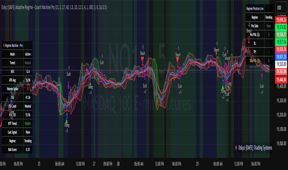
Strategy Stats [presentTrading]Hello! it's another weekend. This tool is a strategy performance analysis tool. Looking at the TradingView community, it seems few creators focus on this aspect. I've intentionally created a shared version. Welcome to share your idea or question on this.
█ Introduction and How it is Different
Strategy Stats is a comprehensive performance analytics framework designed specifically for trading strategies. Unlike standard strategy backtesting tools that simply show cumulative profits, this analytics suite provides real-time, multi-timeframe statistical analysis of your trading performance.
Multi-timeframe analysis: Automatically tracks performance metrics across the most recent time periods (last 7 days, 30 days, 90 days, 1 year, and 4 years)
Advanced statistical measures: Goes beyond basic metrics to include Information Coefficient (IC) and Sortino Ratio
Real-time feedback: Updates performance statistics with each new trade
Visual analytics: Color-coded performance table provides instant visual feedback on strategy health
Integrated risk management: Implements sophisticated take profit mechanisms with 3-step ATR and percentage-based exits
BTCUSD Performance
The table in the upper right corner is a comprehensive performance dashboard showing trading strategy statistics.
Note: While this presentation uses Vegas SuperTrend as the underlying strategy, this is merely an example. The Stats framework can be applied to any trading strategy. The Vegas SuperTrend implementation is included solely to demonstrate how the analytics module integrates with a trading strategy.
⚠️ Timeframe Limitations
Important: TradingView's backtesting engine has a maximum storage limit of 10,000 bars. When using this strategy stats framework on smaller timeframes such as 1-hour or 2-hour charts, you may encounter errors if your backtesting period is too long.
Recommended Timeframe Usage:
Ideal for: 4H, 6H, 8H, Daily charts and above
May cause errors on: 1H, 2H charts spanning multiple years
Not recommended for: Timeframes below 1H with long history
█ Strategy, How it Works: Detailed Explanation
The Strategy Stats framework consists of three primary components: statistical data collection, performance analysis, and visualization.
🔶 Statistical Data Collection
The system maintains several critical data arrays:
equityHistory: Tracks equity curve over time
tradeHistory: Records profit/loss of each trade
predictionSignals: Stores trade direction signals (1 for long, -1 for short)
actualReturns: Records corresponding actual returns from each trade
For each closed trade, the system captures:
float tradePnL = strategy.closedtrades.profit(tradeIndex)
float tradeReturn = strategy.closedtrades.profit_percent(tradeIndex)
int tradeType = entryPrice < exitPrice ? 1 : -1 // Direction
🔶 Performance Metrics Calculation
The framework calculates several key performance metrics:
Information Coefficient (IC):
The correlation between prediction signals and actual returns, measuring forecast skill.
IC = Correlation(predictionSignals, actualReturns)
Where Correlation is the Pearson correlation coefficient:
Correlation(X,Y) = (nΣXY - ΣXY) / √
Sortino Ratio:
Measures risk-adjusted return focusing only on downside risk:
Sortino = (Avg_Return - Risk_Free_Rate) / Downside_Deviation
Where Downside Deviation is:
Downside_Deviation = √
R_i represents individual returns, T is the target return (typically the risk-free rate), and n is the number of observations.
Maximum Drawdown:
Tracks the largest percentage drop from peak to trough:
DD = (Peak_Equity - Trough_Equity) / Peak_Equity * 100
🔶 Time Period Calculation
The system automatically determines the appropriate number of bars to analyze for each timeframe based on the current chart timeframe:
bars_7d = math.max(1, math.round(7 * barsPerDay))
bars_30d = math.max(1, math.round(30 * barsPerDay))
bars_90d = math.max(1, math.round(90 * barsPerDay))
bars_365d = math.max(1, math.round(365 * barsPerDay))
bars_4y = math.max(1, math.round(365 * 4 * barsPerDay))
Where barsPerDay is calculated based on the chart timeframe:
barsPerDay = timeframe.isintraday ?
24 * 60 / math.max(1, (timeframe.in_seconds() / 60)) :
timeframe.isdaily ? 1 :
timeframe.isweekly ? 1/7 :
timeframe.ismonthly ? 1/30 : 0.01
🔶 Visual Representation
The system presents performance data in a color-coded table with intuitive visual indicators:
Green: Excellent performance
Lime: Good performance
Gray: Neutral performance
Orange: Mediocre performance
Red: Poor performance
█ Trade Direction
The Strategy Stats framework supports three trading directions:
Long Only: Only takes long positions when entry conditions are met
Short Only: Only takes short positions when entry conditions are met
Both: Takes both long and short positions depending on market conditions
█ Usage
To effectively use the Strategy Stats framework:
Apply to existing strategies: Add the performance tracking code to any strategy to gain advanced analytics
Monitor multiple timeframes: Use the multi-timeframe analysis to identify performance trends
Evaluate strategy health: Review IC and Sortino ratios to assess predictive power and risk-adjusted returns
Optimize parameters: Use performance data to refine strategy parameters
Compare strategies: Apply the framework to multiple strategies to identify the most effective approach
For best results, allow the strategy to generate sufficient trade history for meaningful statistical analysis (at least 20-30 trades).
█ Default Settings
The default settings have been carefully calibrated for cryptocurrency markets:
Performance Tracking:
Time periods: 7D, 30D, 90D, 1Y, 4Y
Statistical measures: Return, Win%, MaxDD, IC, Sortino Ratio
IC color thresholds: >0.3 (green), >0.1 (lime), <-0.1 (orange), <-0.3 (red)
Sortino color thresholds: >1.0 (green), >0.5 (lime), <0 (red)
Multi-Step Take Profit:
ATR multipliers: 2.618, 5.0, 10.0
Percentage levels: 3%, 8%, 17%
Short multiplier: 1.5x (makes short take profits more aggressive)
Stop loss: 20%

MA Crossover with Demand/Supply Zones + Stop Loss/Take ProfitStop Loss and Take Profit Inputs:
Added stopLossPerc and takeProfitPerc as inputs to allow the user to define the stop loss and take profit levels as a percentage of the entry price.
Stop Loss and Take Profit Calculation:
For long positions, the stop loss is calculated as strategy.position_avg_price * (1 - stopLossPerc), and the take profit is calculated as strategy.position_avg_price * (1 + takeProfitPerc).
For short positions, the stop loss is calculated as strategy.position_avg_price * (1 + stopLossPerc), and the take profit is calculated as strategy.position_avg_price * (1 - takeProfitPerc).
Exit Strategy:
Added strategy.exit to define the stop loss and take profit levels for each trade. The from_entry parameter ensures that the exit is tied to the specific entry order.
Flexibility:
The stop loss and take profit levels are dynamic and adjust based on the entry price of the trade.
How It Works:
When a buy signal is generated (MA crossover near a demand zone), the strategy enters a long position and sets a stop loss and take profit level based on the input percentages.
When a sell signal is generated (MA crossunder near a supply zone), the strategy enters a short position and sets a stop loss and take profit level based on the input percentages.
The trade will exit automatically if either the stop loss or take profit level is hit.
Example:
If the entry price for a long position is $100, and the stop loss is set to 1% while the take profit is set to 2%:
Stop loss level =
100
∗
(
1
−
0.01
)
=
100∗(1−0.01)=99
Take profit level =
100
∗
(
1
+
0.02
)
=
100∗(1+0.02)=102
Notes:
You can adjust the stopLossPerc and takeProfitPerc inputs to suit your risk management preferences.
Always backtest the strategy to ensure the stop loss and take profit levels are appropriate for your trading instrument and timeframe.

Varanormal Mac N Cheez Strategy v1Mac N Cheez Strategy (Set a $200 Take profit Manually)
It's super cheesy. Strategy does the following:
Here's a detailed explanation of what the entire script does, including its key components, functionality, and purpose.
1. Strategy Setup and Input Parameters:
Strategy Name: The script is named "NQ Futures $200/day Strategy" and is set as an overlay, meaning all elements (like moving averages and signals) are plotted on the price chart.
Input Parameters:
fastLength: This sets the length of the fast moving average. The user can adjust this value, and it defaults to 9.
slowLength: This sets the length of the slow moving average. The user can adjust this value, and it defaults to 21.
dailyTarget: The daily profit target, which defaults to $200. If set to 0, this disables the daily profit target.
stopLossAmount: The fixed stop-loss amount per trade, defaulting to $100. This value is used to calculate how much you're willing to lose on a single trade.
trailOffset: This value sets the distance for a trailing stop. It helps protect profits by automatically adjusting the stop-loss as the price moves in your favor.
2. Calculating the Moving Averages:
fastMA: The fast moving average is calculated using the ta.sma() function on the close price with a period length of fastLength. The ta.sma() function calculates the simple moving average.
slowMA: The slow moving average is also calculated using ta.sma() but with the slowLength period.
These moving averages are used to determine trend direction and identify entry points.
3. Buy and Sell Signal Conditions:
longCondition: This is the buy condition. It occurs when the fast moving average crosses above the slow moving average. The script uses ta.crossover() to detect this crossover event.
shortCondition: This is the sell condition. It occurs when the fast moving average crosses below the slow moving average. The script uses ta.crossunder() to detect this crossunder event.
4. Executing Buy and Sell Orders:
Buy Orders: When the longCondition is true (i.e., fast MA crosses above slow MA), the script enters a long position using strategy.entry("Buy", strategy.long).
Sell Orders: When the shortCondition is true (i.e., fast MA crosses below slow MA), the script enters a short position using strategy.entry("Sell", strategy.short).
5. Setting Stop Loss and Trailing Stop:
Stop-Loss for Long Positions: The stop-loss is calculated as the entry price minus the stopLossAmount. If the price falls below this level, the trade is exited automatically.
Stop-Loss for Short Positions: The stop-loss is calculated as the entry price plus the stopLossAmount. If the price rises above this level, the short trade is exited.
Trailing Stop: The trail_offset dynamically adjusts the stop-loss as the price moves in favor of the trade, locking in profits while still allowing room for market fluctuations.
6. Conditional Daily Profit Target:
The script includes a daily profit target that automatically closes all trades once the total profit for the day reaches or exceeds the dailyTarget.
Conditional Logic:
If the dailyTarget is greater than 0, the strategy checks whether the strategy.netprofit (total profit for the day) has reached or exceeded the target.
If the strategy.netprofit >= dailyTarget, the script calls strategy.close_all(), closing all open trades for the day and stopping further trading.
If dailyTarget is set to 0, this logic is skipped, and the script continues trading without a daily profit target.
7. Plotting Moving Averages:
plot(fastMA): This plots the fast moving average as a blue line on the price chart.
plot(slowMA): This plots the slow moving average as a red line on the price chart. These help visualize the crossover points and the trend direction on the chart.
8. Plotting Buy and Sell Signals:
plotshape(): The script uses plotshape() to add visual markers when buy or sell conditions are met:
"Long Signal": When a buy condition (longCondition) is met, a green marker is plotted below the price bar with the label "Long".
"Short Signal": When a sell condition (shortCondition) is met, a red marker is plotted above the price bar with the label "Short".
These markers help traders quickly see when buy or sell signals occurred on the chart.
In addition, triangle markers are plotted:
Green Triangle: Indicates where a buy entry occurred.
Red Triangle: Indicates where a sell entry occurred.
Summary of What the Script Does:
Inputs: The script allows the user to adjust moving average lengths, daily profit targets, stop-loss amounts, and trailing stop offsets.
Signals: It generates buy and sell signals based on the crossovers of the fast and slow moving averages.
Order Execution: It executes long positions on buy signals and short positions on sell signals.
Stop-Loss and Trailing Stop: It sets dynamic stop-losses and uses a trailing stop to protect profits.
Daily Profit Target: The strategy stops trading for the day once the net profit reaches the daily target (unless the target is disabled by setting it to 0).
Visual Markers: It plots moving averages and buy/sell signals directly on the main price chart to aid in visual analysis.
This script is designed to trade based on moving average crossovers, with robust risk management features like stop-loss and trailing stops, along with an optional daily profit target to limit daily trading activity. Let me know if you need further clarification or want to adjust any specific part of the script!

Monthly Purchase Strategy with Dynamic Contract Size This trading strategy is designed to automate monthly purchases of a security, adjusting the size of each purchase based on the percentage of the portfolio's equity. The key features of this strategy include:
Monthly Purchases: The strategy buys the security on a specified day of each month, based on the user's input.
Dynamic Position Sizing: The size of each purchase is calculated as a percentage of the current equity. This allows the position size to adjust dynamically with the portfolio's performance.
Slippage and Commission Considerations: Slippage is simulated by adjusting the entry price by a set number of ticks, while commissions are factored in as fixed costs per trade.
Drawdown Calculation: The strategy tracks the highest equity value and calculates the drawdown, which is the percentage decrease from this peak equity. This helps in assessing the performance and risk of the strategy.
Benefits of the Strategy
Automated Investment: The strategy automates the investment process, reducing the need for manual trading decisions and ensuring consistent execution.
Dynamic Position Sizing: By adjusting the purchase size based on the portfolio’s equity, the strategy helps in managing risk and capitalizing on market movements proportionally to the portfolio’s performance.
Regular Investments: Investing on a regular schedule helps in averaging the purchase price of the security, which can reduce the impact of short-term volatility.
Risk Management: Monitoring drawdown helps in assessing the risk and performance of the strategy, providing insights into potential losses relative to the highest equity value.
Scientific Documentation on ETF Savings Plans
1. Dollar-Cost Averaging and Investment Behavior:
Title: "The Benefits of Dollar-Cost Averaging: A Study of Investment Behavior"
Authors: William F. Sharpe
Journal: Financial Analysts Journal, 1994
Summary: This study discusses the concept of dollar-cost averaging (DCA), which involves investing a fixed amount of money at regular intervals regardless of market conditions. The study highlights that DCA can reduce the impact of market volatility and lower the average cost of investments over time.
Reference: Sharpe, W. F. (1994). The Benefits of Dollar-Cost Averaging: A Study of Investment Behavior. Financial Analysts Journal, 50(4), 27-36.
2. ETFs and Long-Term Investment Strategies:
Title: "Exchange-Traded Funds and Their Role in Long-Term Investment Strategies"
Authors: John C. Bogle
Journal: The Journal of Portfolio Management, 2007
Summary: This paper explores the advantages of using ETFs for long-term investment strategies, emphasizing their low costs, tax efficiency, and diversification benefits. It also discusses how ETFs can be used effectively in automated investment plans like ETF savings plans.
Reference: Bogle, J. C. (2007). Exchange-Traded Funds and Their Role in Long-Term Investment Strategies. The Journal of Portfolio Management, 33(4), 14-25.
3. Risk and Return in ETF Investments:
Title: "Risk and Return Characteristics of Exchange-Traded Funds"
Authors: Eugene F. Fama and Kenneth R. French
Journal: Journal of Financial Economics, 2010
Summary: Fama and French analyze the risk and return characteristics of ETFs compared to traditional mutual funds. The study provides insights into how ETFs can be a viable option for investors seeking diversified exposure while managing risk and optimizing returns.
Reference: Fama, E. F., & French, K. R. (2010). Risk and Return Characteristics of Exchange-Traded Funds. Journal of Financial Economics, 96(2), 257-278.
4. The Impact of Automated Investment Plans:
Title: "The Impact of Automated Investment Plans on Portfolio Performance"
Authors: David G. Blanchflower and Andrew J. Oswald
Journal: Journal of Behavioral Finance, 2012
Summary: This research examines how automated investment plans, including ETF savings plans, affect portfolio performance. It highlights the benefits of automation in reducing behavioral biases and ensuring consistent investment practices.
Reference: Blanchflower, D. G., & Oswald, A. J. (2012). The Impact of Automated Investment Plans on Portfolio Performance. Journal of Behavioral Finance, 13(2), 77-89.
Summary
The "Monthly Purchase Strategy with Dynamic Contract Size and Drawdown" provides a disciplined approach to investing by automating purchases and adjusting position sizes based on portfolio equity. It leverages the benefits of dollar-cost averaging and regular investment, with risk management through drawdown monitoring. Scientific literature supports the effectiveness of ETF savings plans and automated investment strategies in optimizing returns and managing investment risk.

Bollinger Bands Enhanced StrategyOverview
The common practice of using Bollinger bands is to use it for building mean reversion or squeeze momentum strategies. In the current script Bollinger Bands Enhanced Strategy we are trying to combine the strengths of both strategies types. It utilizes Bollinger Bands indicator to buy the local dip and activates trailing profit system after reaching the user given number of Average True Ranges (ATR). Also it uses 200 period EMA to filter trades only in the direction of a trend. Strategy can execute only long trades.
Unique Features
Trailing Profit System: Strategy uses user given number of ATR to activate trailing take profit. If price has already reached the trailing profit activation level, scrip will close long trade if price closes below Bollinger Bands middle line.
Configurable Trading Periods: Users can tailor the strategy to specific market windows, adapting to different market conditions.
Major Trend Filter: Strategy utilizes 100 period EMA to take trades only in the direction of a trend.
Flexible Risk Management: Users can choose number of ATR as a stop loss (by default = 1.75) for trades. This is flexible approach because ATR is recalculated on every candle, therefore stop-loss readjusted to the current volatility.
Methodology
First of all, script checks if currently price is above the 200-period exponential moving average EMA. EMA is used to establish the current trend. Script will take long trades on if this filtering system showing us the uptrend. Then the strategy executes the long trade if candle’s low below the lower Bollinger band. To calculate the middle Bollinger line, we use the standard 20-period simple moving average (SMA), lower band is calculated by the substruction from middle line the standard deviation multiplied by user given value (by default = 2).
When long trade executed, script places stop-loss at the price level below the entry price by user defined number of ATR (by default = 1.75). This stop-loss level recalculates at every candle while trade is open according to the current candle ATR value. Also strategy set the trailing profit activation level at the price above the position average price by user given number of ATR (by default = 2.25). It is also recalculated every candle according to ATR value. When price hit this level script plotted the triangle with the label “Strong Uptrend” and start trail the price at the middle Bollinger line. It also started to be plotted as a green line.
When price close below this trailing level script closes the long trade and search for the next trade opportunity.
Risk Management
The strategy employs a combined and flexible approach to risk management:
It allows positions to ride the trend as long as the price continues to move favorably, aiming to capture significant price movements. It features a user-defined ATR stop loss parameter to mitigate risks based on individual risk tolerance. By default, this stop-loss is set to a 1.75*ATR drop from the entry point, but it can be adjusted according to the trader's preferences.
There is no fixed take profit, but strategy allows user to define user the ATR trailing profit activation parameter. By default, this stop-loss is set to a 2.25*ATR growth from the entry point, but it can be adjusted according to the trader's preferences.
Justification of Methodology
This strategy leverages Bollinger bangs indicator to open long trades in the local dips. If price reached the lower band there is a high probability of bounce. Here is an issue: during the strong downtrend price can constantly goes down without any significant correction. That’s why we decided to use 200-period EMA as a trend filter to increase the probability of opening long trades during major uptrend only.
Usually, Bollinger Bands indicator is using for mean reversion or breakout strategies. Both of them have the disadvantages. The mean reversion buys the dip, but closes on the return to some mean value. Therefore, it usually misses the major trend moves. The breakout strategies usually have the issue with too high buy price because to have the breakout confirmation price shall break some price level. Therefore, in such strategies traders need to set the large stop-loss, which decreases potential reward to risk ratio.
In this strategy we are trying to combine the best features of both types of strategies. Script utilizes ate ATR to setup the stop-loss and trailing profit activation levels. ATR takes into account the current volatility. Therefore, when we setup stop-loss with the user-given number of ATR we increase the probability to decrease the number of false stop outs. The trailing profit concept is trying to add the beat feature from breakout strategies and increase probability to stay in trade while uptrend is developing. When price hit the trailing profit activation level, script started to trail the price with middle line if Bollinger bands indicator. Only when candle closes below the middle line script closes the long trade.
Backtest Results
Operating window: Date range of backtests is 2020.10.01 - 2024.07.01. It is chosen to let the strategy to close all opened positions.
Commission and Slippage: Includes a standard Binance commission of 0.1% and accounts for possible slippage over 5 ticks.
Initial capital: 10000 USDT
Percent of capital used in every trade: 30%
Maximum Single Position Loss: -9.78%
Maximum Single Profit: +25.62%
Net Profit: +6778.11 USDT (+67.78%)
Total Trades: 111 (48.65% win rate)
Profit Factor: 2.065
Maximum Accumulated Loss: 853.56 USDT (-6.60%)
Average Profit per Trade: 61.06 USDT (+1.62%)
Average Trade Duration: 76 hours
These results are obtained with realistic parameters representing trading conditions observed at major exchanges such as Binance and with realistic trading portfolio usage parameters.
How to Use
Add the script to favorites for easy access.
Apply to the desired timeframe and chart (optimal performance observed on 4h BTC/USDT).
Configure settings using the dropdown choice list in the built-in menu.
Set up alerts to automate strategy positions through web hook with the text: {{strategy.order.alert_message}}
Disclaimer:
Educational and informational tool reflecting Skyrex commitment to informed trading. Past performance does not guarantee future results. Test strategies in a simulated environment before live implementation

[imba]lance algo🟩 INTRODUCTION
Hello, everyone!
Please take the time to review this description and source code to utilize this script to its fullest potential.
🟩 CONCEPTS
This is a trend indicator. The trend is the 0.5 fibonacci level for a certain period of time.
A trend change occurs when at least one candle closes above the level of 0.236 (for long) or below 0.786 (for short). Also it has massive amout of settings and features more about this below.
With good settings, the indicator works great on any market and any time frame!
A distinctive feature of this indicator is its backtest panel. With which you can dynamically view the results of setting up a strategy such as profit, what the deposit size is, etc.
Please note that the profit is indicated as a percentage of the initial deposit. It is also worth considering that all profit calculations are based on the risk % setting.
🟩 FEATURES
First, I want to show you what you see on the chart. And I’ll show you everything closer and in more detail.
1. Position
2. Statistic panel
3. Backtest panel
Indicator settings:
Let's go in order:
1. Strategies
This setting is responsible for loading saved strategies. There are only two preset settings, MANUAL and UNIVERSAL. If you choose any strategy other than MANUAL, then changing the settings for take profits, stop loss, sensitivity will not bring any results.
You can also save your customized strategies, this is discussed in a separate paragraph “🟩HOW TO SAVE A STRATEGY”
2. Sensitive
Responsible for the time period in bars to create Fibonacci levels
3. Start calculating date
This is the time to start backtesting strategies
4. Position group
Show checkbox - is responsible for displaying positions
Fill checkbox - is responsible for filling positions with background
Risk % - is responsible for what percentage of the deposit you are willing to lose if there is a stop loss
BE target - here you can choose when you reach which take profit you need to move your stop loss to breakeven
Initial deposit- starting deposit for profit calculation
5. Stoploss group
Fixed stoploss % checkbox - If choosed: stoploss will be calculated manually depending on the setting below( formula: entry_price * (1 - stoploss percent)) If NOT choosed: stoploss will be ( formula: fibonacci level(0.786/0.236) * (1 + stoploss percent))
6. Take profit group
This group of settings is responsible for how far from the entry point take profits will be and what % of the position to fix
7. RSI
Responsible for configuring the built-in RSI. Suitable bars will be highlighted with crosses above or below, depending on overbought/oversold
8. Infopanels group
Here I think everything is clear, you can hide or show information panels
9. Developer mode
If enabled, all events that occur will be shown, for example, reaching a take profit or stop loss with detailed information about the unfixed balance of the position
🟩 HOW TO USE
Very simple. All you need is to wait for the trend to change to long or short, you will immediately see a stop loss and four take profits, and you will also see prices. Like in this picture:
🟩 ALERTS
There are 3 types of alerts:
1. Long signal
2. Short signal
3. Any alert() function call - will be send to you json with these fields
{
"side": "LONG",
"entry": "64.454",
"tp1": "65.099",
"tp2": "65.743",
"tp3": "66.388",
"tp4": "67.032",
"winrate": "35.42%",
"strategy": "MANUAL",
"beTargetTrigger": "1",
"stop": "64.44"
}
🟩 HOW TO SAVE A STRATEGY
First, you need to make sure that the “MANUAL” strategy is selected in the strategy settings.
After this, you can start selecting parameters that will show the largest profit in the statistics panel.
I have highlighted what you need to pay attention to when choosing a strategy
Let's assume you have set up a strategy. The main question is how to preserve it?
Let’s say the strategy turned out with the following parameters:
Next we need to find this section of code:
// STRATS
selector(string strategy_name) =>
strategy_settings = Strategy_settings.new()
switch strategy_name
"MANUAL" =>
strategy_settings.sensitivity := 18
strategy_settings.risk_percent := 1
strategy_settings.break_even_target := "1"
strategy_settings.tp1_percent := 1
strategy_settings.tp1_percent_fix := 40
strategy_settings.tp2_percent := 2
strategy_settings.tp2_percent_fix := 30
strategy_settings.tp3_percent := 3
strategy_settings.tp3_percent_fix := 20
strategy_settings.tp4_percent := 4
strategy_settings.tp4_percent_fix := 10
strategy_settings.fixed_stop := false
strategy_settings.sl_percent := 0.0
"UNIVERSAL" =>
strategy_settings.sensitivity := 20
strategy_settings.risk_percent := 1
strategy_settings.break_even_target := "1"
strategy_settings.tp1_percent := 1
strategy_settings.tp1_percent_fix := 40
strategy_settings.tp2_percent := 2
strategy_settings.tp2_percent_fix := 30
strategy_settings.tp3_percent := 3
strategy_settings.tp3_percent_fix := 20
strategy_settings.tp4_percent := 4
strategy_settings.tp4_percent_fix := 10
strategy_settings.fixed_stop := false
strategy_settings.sl_percent := 0.0
// "NEW STRATEGY" =>
// strategy_settings.sensitivity := 20
// strategy_settings.risk_percent := 1
// strategy_settings.break_even_target := "1"
// strategy_settings.tp1_percent := 1
// strategy_settings.tp1_percent_fix := 40
// strategy_settings.tp2_percent := 2
// strategy_settings.tp2_percent_fix := 30
// strategy_settings.tp3_percent := 3
// strategy_settings.tp3_percent_fix := 20
// strategy_settings.tp4_percent := 4
// strategy_settings.tp4_percent_fix := 10
// strategy_settings.fixed_stop := false
// strategy_settings.sl_percent := 0.0
strategy_settings
// STRATS
Let's uncomment on the latest strategy called "NEW STRATEGY" rename it to "SOL 5m" and change the sensitivity:
// STRATS
selector(string strategy_name) =>
strategy_settings = Strategy_settings.new()
switch strategy_name
"MANUAL" =>
strategy_settings.sensitivity := 18
strategy_settings.risk_percent := 1
strategy_settings.break_even_target := "1"
strategy_settings.tp1_percent := 1
strategy_settings.tp1_percent_fix := 40
strategy_settings.tp2_percent := 2
strategy_settings.tp2_percent_fix := 30
strategy_settings.tp3_percent := 3
strategy_settings.tp3_percent_fix := 20
strategy_settings.tp4_percent := 4
strategy_settings.tp4_percent_fix := 10
strategy_settings.fixed_stop := false
strategy_settings.sl_percent := 0.0
"UNIVERSAL" =>
strategy_settings.sensitivity := 20
strategy_settings.risk_percent := 1
strategy_settings.break_even_target := "1"
strategy_settings.tp1_percent := 1
strategy_settings.tp1_percent_fix := 40
strategy_settings.tp2_percent := 2
strategy_settings.tp2_percent_fix := 30
strategy_settings.tp3_percent := 3
strategy_settings.tp3_percent_fix := 20
strategy_settings.tp4_percent := 4
strategy_settings.tp4_percent_fix := 10
strategy_settings.fixed_stop := false
strategy_settings.sl_percent := 0.0
"SOL 5m" =>
strategy_settings.sensitivity := 15
strategy_settings.risk_percent := 1
strategy_settings.break_even_target := "1"
strategy_settings.tp1_percent := 1
strategy_settings.tp1_percent_fix := 40
strategy_settings.tp2_percent := 2
strategy_settings.tp2_percent_fix := 30
strategy_settings.tp3_percent := 3
strategy_settings.tp3_percent_fix := 20
strategy_settings.tp4_percent := 4
strategy_settings.tp4_percent_fix := 10
strategy_settings.fixed_stop := false
strategy_settings.sl_percent := 0.0
strategy_settings
// STRATS
Now let's find this code:
strategy_input = input.string(title = "STRATEGY", options = , defval = "MANUAL", tooltip = "EN:\nTo manually configure the strategy, select MANUAL otherwise, changing the settings won't have any effect\nRU:\nЧтобы настроить стратегию вручную, выберите MANUAL в противном случае изменение настроек не будет иметь никакого эффекта")
And let's add our new strategy there, it turned out like this:
strategy_input = input.string(title = "STRATEGY", options = , defval = "MANUAL", tooltip = "EN:\nTo manually configure the strategy, select MANUAL otherwise, changing the settings won't have any effect\nRU:\nЧтобы настроить стратегию вручную, выберите MANUAL в противном случае изменение настроек не будет иметь никакого эффекта")
That's all. Our new strategy is now saved! It's simple! Now we can select it in the list of strategies:
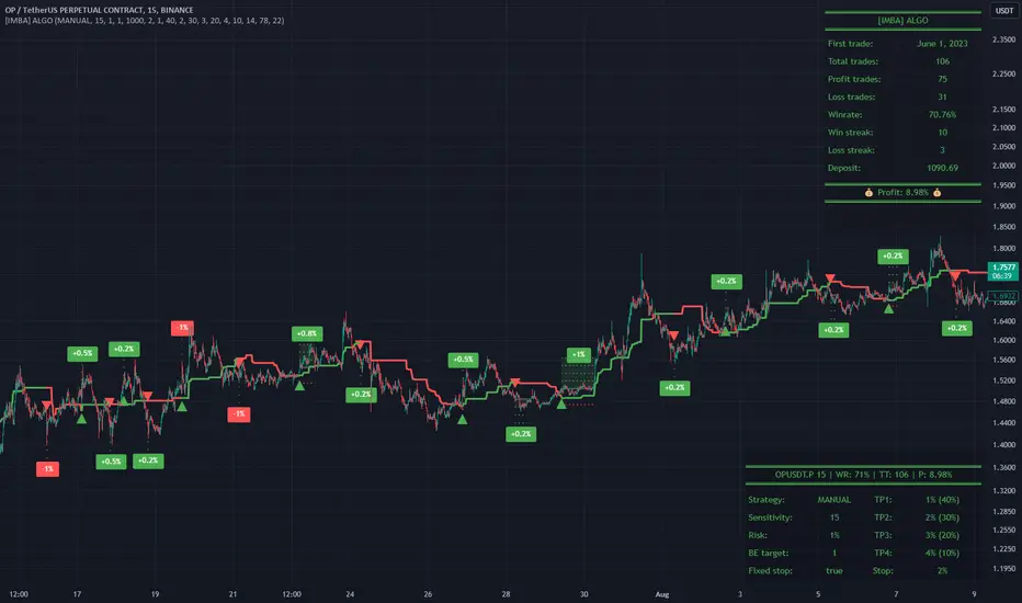
Goldmine Wealth Builder - DKK/SKKGoldmine Wealth Builder
Version 1.0
Introduction to Long-Term Investment Strategies: DKK, SKK1 and SKK2
In the dynamic realm of long-term investing, the DKK, SKK1, and SKK2 strategies stand as valuable pillars. These strategies, meticulously designed to assist investors in building robust portfolios, combine the power of Super Trend, RSI (Relative Strength Index), Exponential Moving Averages (EMAs), and their crossovers. By providing clear alerts and buy signals on a daily time frame, they equip users with the tools needed to make well-informed investment decisions and navigate the complexities of the financial markets. These strategies offer a versatile and structured approach to both conservative and aggressive investment, catering to the diverse preferences and objectives of investors.
Each part of this strategy provides a unique perspective and approach to the accumulation of assets, making it a versatile and comprehensive method for investors seeking to optimize their portfolio performance. By diligently applying this multi-faceted approach, investors can make informed decisions and effectively capitalize on potential market opportunities.
DKK Strategy for ETFs and Funds:
The DKK system is a strategy designed for accumulating ETFs and Funds as long-term investments in your portfolio. It simplifies the process of identifying trend reversals and opportune moments to invest in listed ETFs and Funds, particularly during bull markets. Here's a detailed explanation of the DKK system:
Objective: The primary aim of the DKK system is to build a long-term investment portfolio by focusing on ETFs and Funds. It facilitates the identification of stocks that are in the process of reversing their trends, allowing investors to benefit from upward price movements in these financial instruments.
Stock Selection Criteria: The DKK system employs specific criteria for selecting ETFs and Funds:
• 200EMA (Exponential Moving Average): The system monitors whether the prices of ETFs and Funds are consistently below the 200-day Exponential Moving Average. This is considered an indicator of weakness, especially on a daily time frame.
• RSI (Relative Strength Index): The system looks for an RSI value of less than 40. An RSI below 40 is often seen as an indication of a weak or oversold condition in a financial instrument.
Alert Signal: Once the DKK system identifies ETFs and Funds meeting these criteria, it provides an alert signal:
• Red Upside Triangle Sign: This signal is automatically generated on the daily chart of ETFs and Funds. It serves as a clear indicator to investors that it's an opportune time to accumulate these financial instruments for long-term investment.
It's important to note that the DKK system is specifically designed for ETFs and Funds, so it should be applied to these types of investments. Additionally, it's recommended to track index ETFs and specific types of funds, such as REITs (Real Estate Investment Trusts) and INVITs (Infrastructure Investment Trusts), in line with the DKK system's approach. This strategy simplifies the process of identifying investment opportunities within this asset class, particularly during periods of market weakness.
SKK1 Strategy for Conservative Stock Investment:
The SKK 1 system is a stock investment strategy tailored for conservative investors seeking long-term portfolio growth with a focus on stability and prudent decision-making. This strategy is meticulously designed to identify pivotal market trends and stock price movements, allowing investors to make informed choices and capitalize on upward market trends while minimizing risk. Here's a comprehensive overview of the SKK 1 system, emphasizing its suitability for conservative investors:
Objective: The primary objective of the SKK 1 system is to accumulate stocks as long-term investments in your portfolio while prioritizing capital preservation. It offers a disciplined approach to pinpointing potential entry points for stocks, particularly during market corrections and trend reversals, thereby enabling you to actively participate in bullish market phases while adopting a conservative risk management stance.
Stock Selection Criteria: The SKK 1 system employs a stringent set of criteria to select stocks for investment:
• Correction Mode: It identifies stocks that have undergone a correction, signifying a decline in stock prices from their recent highs. This conservative approach emphasizes the importance of seeking stocks with a history of stability.
• 200EMA (Exponential Moving Average): The system diligently analyses daily stock price movements, specifically looking for stocks that have fallen to or below the 200-day Exponential Moving Average. This indicator suggests potential overselling and aligns with a conservative strategy of buying low.
Trend Reversal Confirmation: The SKK 1 system doesn't merely pinpoint stocks in correction mode; it takes an extra step to confirm a trend reversal. It employs the following indicators:
• Short-term Downtrends Reversal: This aspect focuses on identifying the reversal of short-term downtrends in stock prices, observed through the transition of the super trend indicator from the red zone to the green zone. This cautious approach ensures that the trend is genuinely shifting.
• Super Trend Zones: These zones are crucial for assessing whether a stock is in a bullish or bearish trend. The system consistently monitors these zones to confirm a potential trend reversal.
Alert & Buy Signals: When the SKK 1 system identifies stocks that have reached a potential bottom and are on the verge of a trend reversal, it issues vital alert signals, aiding conservative investors in prudent decision-making:
• Orange Upside Triangle Sign: This signal serves as a cautious heads-up, indicating that a stock may be poised for a trend reversal. It advises investors to prepare funds for potential investment without taking undue risks.
• Green Upside Triangle Sign: This is the confirmation of a trend reversal, signifying a robust buy signal. Conservative investors can confidently enter the market at this point, accumulating stocks for a long-term investment, secure in the knowledge that the trend is in their favor.
In summary, the SKK 1 system is a systematic and conservative approach to stock investing. It excels in identifying stocks experiencing corrections and ensures that investors act when there's a strong indication of a trend reversal, all while prioritizing capital preservation and risk management. This strategy empowers conservative investors to navigate the intricacies of the stock market with confidence, providing a calculated and stable path toward long-term portfolio growth.
Note: The SKK1 strategy, known for its conservative approach to stock investment, also provides an option to extend its methodology to ETFs and Funds for those investors who wish to accumulate assets more aggressively. By enabling this feature in the settings, you can harness the SKK1 strategy's careful criteria and signal indicators to accumulate aggressive investments in ETFs and Funds.
This flexible approach acknowledges that even within a conservative strategy, there may be opportunities for more assertive investments in assets like ETFs and Funds. By making use of this option, you can strike a balance between a conservative stance in your stock portfolio while exploring an aggressive approach in other asset classes. It offers the versatility to cater to a variety of investment preferences, ensuring that you can adapt your strategy to suit your financial goals and risk tolerance.
SKK 2 Strategy for Aggressive Stock Investment:
The SKK 2 strategy is designed for those who are determined not to miss significant opportunities within a continuous uptrend and seek a way to enter a trend that doesn't present entry signals through the SKK 1 strategy. While it offers a more aggressive entry approach, it is ideal for individuals willing to take calculated risks to potentially reap substantial long-term rewards. This strategy is particularly suitable for accumulating stocks for aggressive long-term investment. Here's a detailed description of the SKK 2 strategy:
Objective: The primary aim of the SKK 2 strategy is to provide an avenue for investors to identify short-term trend reversals and seize the opportunity to enter stocks during an uptrend, thereby capitalizing on a sustained bull run. It acknowledges that there may not always be clear entry signals through the SKK 1 strategy and offers a more aggressive alternative.
Stock Selection Criteria: The SKK 2 strategy utilizes a specific set of criteria for stock selection:
1. 50EMA (Exponential Moving Average): It targets stocks that are trading below the 50-day Exponential Moving Average. This signals a short-term reversal from the top and indicates that the stock is in a downtrend.
2. RSI (Relative Strength Index): The strategy considers stocks with an RSI of less than 40, which is an indicator of weakness in the stock.
Alert Signals: The SKK 2 strategy provides distinct alert signals that facilitate entry during an aggressive reversal:
• Red Downside Triangle Sign: This signal is triggered when the stock is below the 50EMA and has an RSI of less than 40. It serves as a clear warning of a short-term reversal from the top and a downtrend, displayed on the daily chart.
• Purple Upside Triangle Sign: This sign is generated when a reversal occurs through a bullish candle, and the RSI is greater than 40. It signifies the stock has bottomed out from a short-term downtrend and is now reversing. This purple upside triangle serves as an entry signal on the chart, presenting an attractive opportunity to accumulate stocks during a strong bullish phase, offering a chance to seize a potentially favorable long-term investment.
In essence, the SKK 2 strategy caters to aggressive investors who are willing to take calculated risks to enter stocks during a continuous uptrend. It focuses on identifying short-term reversals and provides well-defined signals for entry. While this strategy is more aggressive in nature, it has the potential to yield substantial rewards for those who are comfortable with a higher level of risk and are looking for opportunities to build a strong long-term portfolio.
Introduction to Strategy Signal Information Chart
This chart provides essential information on strategy signals for DKK, SKK1, and SKK2. By quickly identifying "Buy" and "Alert" signals for each strategy, investors can efficiently gauge market conditions and make informed decisions to optimize their investment portfolios.
In Conclusion
These investment strategies, whether conservative like DKK and SKK1 or more aggressive like SKK2, offer a range of options for investors to navigate the complex world of long-term investments. The combination of Super Trend, RSI, and EMAs with their crossovers provides clear signals on a daily time frame, empowering users to make well-informed decisions and potentially capitalize on market opportunities. Whether you're looking for stability or are ready to embrace more risk, these strategies have something to offer for building and growing your investment portfolio.

Previous Day High Low Strategy only for LongWelcome to the "Previous Day High Low Strategy only for Long"!.
This strategy aims to identify potential long trading opportunities based on the previous day's high and low prices, along with certain market strength conditions.
Key Features:
Entry Conditions: The strategy triggers a long position when the current day's closing price crosses above the previous day's high or low.
Market Strength Filter: The strategy incorporates a market strength filter using the Average Directional Index (ADX). It only takes long positions when the ADX value is above a specific threshold and when there is a predominance of upward movement.
Trade Timing: The strategy operates within a specified trade window, starting at 09:30 and ending at 15:10. Positions are closed at 15:15 if still active.
Risk Management: The strategy employs dynamic stop-loss and profit-taking levels based on a user-defined Max Profit value. It has three profit targets (T1, T2, T3) and a stop-loss level to manage risk effectively.
Rules:
Ensure that the strategy idea is clearly understandable. Provide an easy-to-read title and a thoughtful description explaining the reasoning behind the strategy.
All content should be ad-free. Avoid any form of promotion, advertising, or solicitation.
No fundraising requests or money solicitation is allowed on TradingView.
Publish in the same language as the TradingView subdomain you're on, except for script titles, which must be in English.
Don't plagiarize. Create and share only unique content, and always give credit when using someone else's work.
Be respectful, kind, and constructive when engaging with others.
Zero tolerance for contentious political discourse, defamatory, threatening, or discriminatory remarks.
Avoid sharing harmful, misleading, or inappropriate content.
Respect the moderators' work and address complaints privately.
Use only your original account and avoid creating duplicate or fake accounts.
Do not attempt to manipulate the reputation system or engage in like-for-like schemes.
Explanation of how the strategy works
1. Previous Day's High and Low (HH, LL):
In this strategy, we start by obtaining the high and low prices of the previous day (not the current day) using the request.security function. This function allows us to access historical data for a specific time frame. The high and low prices are stored in the variables HH and LL, respectively.
2. Entry Conditions:
The strategy uses two conditions to trigger a long position:
Condition 1 (Long Condition 1): If the closing price of the current day crosses above the previous day's high (HH), it generates a long signal. This is achieved using the ta.crossover function, which detects when a crossover occurs.
Condition 2 (Long Condition 2): Similarly, if the closing price of the current day crosses above the previous day's low (LL), it also generates a long signal.
Combined Condition: To take long positions, the strategy combines both long conditions using the logical OR operator (or). This means that if either of the two conditions is met, a long position will be initiated.
3. Market Strength Filter:
The strategy also includes a filter based on the Average Directional Index (ADX) to gauge the market's strength before taking long positions. The ADX measures the strength of a trend in the market. The higher the ADX value, the stronger the trend.
Calculation of ADX: The ADX is calculated using the adx function, which takes two parameters: LWdilength (DMI Length) and LWadxlength (ADX period).
Strength Condition (strength_up): The strategy requires that the ADX value should be above a threshold (11 in this case) and that there is a predominance of upward movement (up > down) before initiating a long position. The LWADX value is multiplied by 2.5 and compared to the highest value of LWADX from the last 4 periods using ta.highest(LWADX , 4). If these conditions are met, the variable strength_up is set to true.
Combined Condition: The strength_up condition is then combined with the long conditions using the logical AND operator (and). This means that the strategy will only take a long position if both the long conditions and the market strength condition are met.
4. Trade Timing:
The strategy sets a specific trade window between 09:30 and 15:10. It will only execute trades within this time frame (TradeTime).
5. Risk Management:
The strategy implements dynamic stop-loss (SL) and profit-taking levels (T1, T2, T3) based on a user-defined Max Profit value. The stop-loss is set as a percentage of the Max Profit value. As the position moves in favor of the trader, the profit targets are adjusted accordingly.
6. Position Management:
The strategy uses the strategy.entry function to enter long positions based on the combined entry conditions. Once a position is open, the script uses strategy.exit to define the exit condition when either the profit target or stop-loss level is hit. The strategy.close function is used to close any open position at the end of the trade window (15:15).
7. Plotting:
The strategy uses the plot function to visualize the previous day's high and low prices, as well as the stop-loss (SL) and profit-taking (T1, T2, T3) levels on the chart.
Overall, the "Previous Day High Low Strategy only for Long" aims to identify potential long trading opportunities based on the previous day's price action and market strength conditions. However, as with any trading strategy, it's essential to thoroughly test it and consider risk management before applying it to real-world trading scenarios.
Disclaimer:
The information presented by this strategy is for educational purposes only and should not be considered as investment advice. The strategy is not designed for qualified investors. Always conduct your own research and consult with a financial advisor before making any trading decisions.
Remember, the success of any trading strategy depends on various factors, including market conditions, risk management, and individual trading skills. Past performance is not indicative of future results.

Rsi strategy for BTC with (Rsi SPX)
I hope this strategy is just an idea and a starting point, I use the correlation of the Sp500 with the Btc, this does not mean that this correlation will exist forever!. I love Trading view and I'm learning to program, I find correlations very interesting and here is a simple strategy.
This is a trading strategy script written in Pine Script language for use in TradingView. Here is a brief overview of the strategy:
The script uses the RSI (Relative Strength Index) technical indicator with a period of 14 on two securities: the S&P 500 (SPX) and the symbol corresponding to the current chart (presumably Bitcoin, based on the variable name "Btc_1h_fixed"). The RSI is plotted on the chart for both securities.
The script then sets up two trading conditions using the RSI values:
A long entry condition: when the RSI for the current symbol crosses above the RSI for the S&P 500, a long trade is opened using the "strategy.entry" function.
A short entry condition: when the RSI for the current symbol crosses below the RSI for the S&P 500, a short trade is opened using the "strategy.entry" function.
The script also includes a take profit input parameter that allows the user to set a percentage profit target for closing the trade. The take profit is set using the "strategy.exit" function.
Overall, the strategy aims to take advantage of divergences in RSI values between the current symbol and the S&P 500 by opening long or short trades accordingly. The take profit parameter allows the user to set a specific profit target for each trade. However, the script does not include any stop loss or risk management features, which should be considered when implementing the strategy in a real trading scenario.
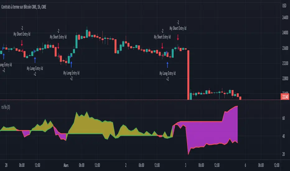
3LS | 3 Line Strike Strategy [Kintsugi Trading]What is the 3LS | 3 Line Strike Strategy?
Incorporating the 3 Line Strike candlestick pattern into our strategy was inspired by Arty at The Moving Average and the amazing traders at TheTrdFloor .
The Three Line Strike is a trend continuation candlestick pattern consisting of four candles. Depending on their heights and collocation, a bullish or a bearish trend continuation can be predicted.
In a symphony of trend analysis, price action, and volume we can find and place high-probability trades with the 3LS Strategy.
How to use it!
----- First, start by choosing a Stop-Loss Strategy, Stop PIP Size, and Risk/Reward Ratio -----
- Stop-Loss Strategy
Fixed PIP Size – This uses the top/bottom of the indicator candle and places a TP based on the chosen Risk:Reward ratio.
ATR Trail (No set Target Profit, only uses ATR Stop)
ATR Trail-Stop (Has set Target Profit, however, stop is based on ATR inputs)
**If you choose an ATR Stop-Loss Strategy - input the desired ATR period and Multiple you would like the stop to be calculated at**
**ATR Stop-Loss Strategies have a unique alert setup for Auto-Trading. See Auto-Trading Section**
- Risk/Reward Ratio = If you have a .5 risk/reward, it means you are risking $100 to make $50.
- Additional Stop PIP Size = Number of PIPs over the default stop location of the top or bottom of the indicator candle.
----- Next, we set the Session Filter -----
Set the Timezone and Trade Session you desire. If no specific session is desired, simply set the Trade Session to 00:00 - 00:00.
----- Next, we set the Moving Average Cloud Fill -----
Enter the Fast and Slow Moving Average Length used to calculate trend direction:
MA Period Fast
MA Period Slow
These inputs will determine whether the strategy looks for Long or Short positions.
----- Next, we set the VSA – Volume Spread Analysis Settings -----
Check the box to show the indicator at the bottom of the chart if desired.
This is just a different visual output of the VSA | Volume Spread Analysis indicator available for free under the community indicators tab. You can add that indicator to your chart and see the same output in candle format.
In combination with the Moving Average Cloud, the Volume Spread Analysis will help us determine when to take a trade and in what direction.
The strategy is essentially looking for small reversals going against the overall trend and placing a trade once that reversal ends and the price moves back in the direction of the overall trend.
The 3LS Strategy utilizes confirmation between trend, volume, and price action to place high probability trades.
The VSA is completely customizable by:
Moving Average Length
MA-1 Multiplier
MA-2 Multiplier
MA-3 Multiplier
Check out the VSA | Volume Spread Analysis indicator in the community scripts section under the indicators tab to use this awesome resource on other strategies.
----- Next, we have the option to view the automated KT Bull/Bear Signals -----
Check the boxes to show the buy-sell signal on the chart if desired.
----- Next, we set the risk we want to use if Auto Trading the strategy -----
I always suggest using no more than 1-3% of your total account balance per trade. Remember, if you have multiple strategies triggering per day with each using 1%, the total percent at risk will be much larger.
For Example – if you have 10 strategies each risking 1% your total risk is 10% of your account, not 1%! Be mindful to only use 1-3% of your total account balance across all strategies, not just each individual one.
----- Finally, we backtest our ideas -----
After using the 'Strategy Tester' tab on TradingView to thoroughly backtest your predictions you are ready to take it to the next level - Automated Trading!
This was my whole reason for creating the script. If you work a full-time job, live in a time zone that is hard to trade, or just don't have the patience, this will be a game-changer for you as it was for me.
Auto-Trading
When it comes to auto-trading this strategy I have included two options in the script that utilize the alert messages generated by TradingView.
*Note: Please trade on a demo account until you feel comfortable enough to use real money, and then please stick to 1%-2% of your total account value in risk per trade.*
AutoView
PineConnector
**ATR Auto-Trading Alert Setup**
How to create alerts on 3 Line Strike Strategy
For Trailing Stops:
1) Adjust autoview/pineconnector settings
2) Click "add alert"
3) Select "Condition" = Strategy Name
4) Select "Order Fills Only" from the drop-down
3) Remove template message text from "message" box and place the exact text. '{{strategy.order.alert_message}}'
4) Click "create"
For Fixed Pip Stop:
1) Adjust autoview/pineconnector settings
2) Click "add alert"
3) Select "Condition" = Strategy Name
4) Select "alert() function calls only"
5) I like to title my Alert Name the same thing I named it as an Indicator Template to keep track
Good luck with your trading!
Template Trailing Strategy (Backtester)💭 Overview
+ Title: Template Trailing Strategy (Backtester)
+ Author: Iason Nikolas (jason5480)
+ License: CC BY-NC-SA 4.0
💢 What is the "Template Trailing Strategy (Backtester)" ❓
The "Template Trailing Strategy (Backtester)" (TTS) is a back-tester orchestration framework. It supercharges the implementation-test-evaluation lifecycle of new trading strategies, by making it possible to plug in your own trading idea.
While TTS offers a vast number of configuration settings, it primarily allows the trader to:
Test and evaluate your own trading logic that is described in terms of entry, exit, and cancellation conditions.
Define the entry and exit order types as well as their target prices when the limit, stop, or stop-limit order types are used.
Utilize a variety of options regarding the placement of the stop-loss and take-profit target(s) prices and support for well-known techniques like moving to breakeven and trailing.
Provide well-known quantity calculation methods to properly handle risk management and easily evaluate trading strategies and compare them.
Alert on each trading event or any related change through a robust and fully customizable messaging system.
All of the above makes TTS a practical toolkit: once you learn it, many repetitive tasks that strategy authors usually re-implement are eliminated. Using TradingView’s built-in backtesting engine makes testing and comparing ideas straightforward.
By utilizing the TTS one can easily swap "trading logic" by testing, evaluating, and comparing each trading idea and/or individual component of a strategy.
Finally, TTS, through its per-event alert management (and debugging) system, provides an automated solution that supports live trading with brokers via webhooks.
NOTE: The "Template Trailing Strategy (Backtester)" does not dictate how you can combine different indicator types. Thus, it should not be confused as a "Trading System", because it gives its user full flexibility on that end (for better or worse).
💢 What is a "Signal Indicator" ❓
"Signal Indicator" (SI) is an indicator that can output a "signal" that follows a specific convention so that the "Template Trailing Strategy (Backtester)" can "understand" and execute the orders accordingly. The SI realizes the core trading logic signaling to the TTS when to enter, exit, or cancel an order. A SI instructs the TTS "when" to enter or exit, and the TTS determines "how" to enter and exit the position once the Signal Indicator generates a signal.
A very simple example of a Signal Indicator might be a 200-day Simple Moving Average Signal. When the price of the security closes above the 200-day SMA, a SI would provide TTS with a "long entry signal". Once TTS receives the "long entry signal", the TTS will open a long position and send an alert or automated trade message via webhook to a broker, based on the Entry settings defined in TTS. If the TTS Entry settings specify a "Market" order type, then the open long position will be executed by TTS immediately. But if the TTS Entry settings specify a "Stop" order type with a 1% Stop Distance, then when the price of the security rises by 1% after the "long entry signal" occurs, the TTS will open a long position and the Long Entry alert or webhook to the broker will be sent.
🤔 How to Guide
💢 How to connect a "signal" from a "Signal Indicator" ❓
The "Template Trailing Strategy (Backtester)" was designed to receive external signals from a "Signal Indicator". In this way, a "new trading idea" can be developed, configured, and evaluated separately from the TTS. Similarly, the SI can be held constant, and the trading mechanics can change in the TTS settings and back-tested to answer questions such as, "Am I better with a different stop loss placement method, what if I used a limit order instead of a stop order to enter, what if I used 25% margin instead of trading spot market?"
To make that possible by connecting an external signal indicator to TTS, you should:
Add both your SI (e.g. "Two MA Signal Indicator" , "Click Signal Indicator" , "Signal Adapter" , "Signal Composer" ) and the TTS script to the same chart.
Open the script's Settings / Inputs dialog for the TTS.
In the 🛠️ STRATEGY group set 𝐃𝐞𝐚𝐥 𝐂𝐨𝐧𝐝𝐢𝐨𝐧𝐬 𝐌𝐨𝐝𝐞 to 🔨External (this makes TTS listen to an external signal source).
Still inside 🛠️ STRATEGY locate the 🔌𝐒𝐢𝐠𝐧𝐚𝐥 🛈 input and choose the plotted output of your SI. The option should look like: "<SI short title>:🔌Signal to TTS" .
Verbose troubleshooting & tips
If the SI does not appear in the 🔌Signal 🛈 selector, confirm both scripts are added to the same chart and the SI exposes a plotted series (title often "🔌Signal to TTS").
When using multiple SIs, pick the SI instance that actually outputs the "🔌Signal to TTS" plotted series.
Validate on the chart: when your SI changes state, the plotted "🔌Signal" series in the TTS (visible in the data window) should change accordingly.
The TTS accepts only signals that follow the tts_convention DealConditions structure. Do not attempt to feed arbitrary scalar series without using conv.getDealConditions / conv.DealConditions.
Make sure your SI composes a DealConditions value following the TTS convention (startLong, endLong, startShort, endShort — optional cancel fields). See the template below.
If the plot is present but TTS does not react, ensure the SI plot is non-repainting (or accept realtime/backtest limitations). Test on historical bars first.
Create alerts on the strategy (see the Alerts section). Use the {{strategy.order.alert_message}} placeholder in the Create Alert dialog to forward TTS messages.
💢 How to create a custom trading logic ❓
The "Template Trailing Strategy (Backtester)" provides two ways to plug in your custom trading logic. Both of them have their advantages and disadvantages.
✍️ Develop your own Customized "Signal Indicator" 💥
The first approach is meant to be used for relatively more complex trading logic. The advantages of this approach are the full control and customization you have over the trading logic and the relatively simple configuration setup by having two scripts only. The downsides are that you have to have some experience with pinescript or you are willing to learn and experiment. You should also know the exact formula for every indicator you will use since you have to write it by yourself. Copy-pasting from existing open-source indicators will get you started quite fast though.
The idea here is either to create a new indicator script from scratch or to copy an existing non-signal indicator and make it a "Signal Indicator". To create a new script, press the "Pine Editor" button below the chart to open the "Pine Editor" and then press the "Open" button to open the drop-down menu with the templates. Select the "New Indicator" option. Add it to your chart to copy an existing indicator and press the source code {} button. Its source code will be shown in the "Pine Editor" with a warning on top stating that this is a read-only script. Press the "create a working copy". Now you can give a descriptive title and a short title to your script, and you can work on (or copy-paste) the (other) indicators of your interest. Once you have the information needed to decide, define a DealConditions object and plot it like this:
import jason5480/tts_convention/ as conv
// Calculate the start, end, cancel start, cancel end conditions
dealConditions = conv.DealConditions.new(
startLongDeal = ,
startShortDeal = ,
endLongDeal = ,
endShortDeal = ,
cnlStartLongDeal = ,
cnlStartShortDeal = ,
cnlEndLongDeal = ,
cnlEndShortDeal = )
// Use this signal in scripts like "Template Trailing Strategy (Backtester)" and "Signal Composer" that can utilize its value
// Emit the current signal value according to the TTS framework convention
plot(series = conv.getSignal(dealConditions), title = '🔌Signal to TTS', color = #808000, editable = false, display = display.data_window + display.status_line, precision = 0)
You should import the latest version of the tts_convention library and write your deal conditions appropriately based on your trading logic and put them in the code section shown above by replacing the "…" part after "=". You can omit the conditions that are not relevant to your logic. For example, if you use only market orders for entering and exiting your positions the cnlStartLongDeal, cnlStartShortDeal, cnlEndLongDeal, and cnlEndShortDeal are irrelevant to your case and can be safely omitted from the DealConditions object. After successfully compiling your new custom SI script add it to the same chart with the TTS by pressing the "Add to chart" button. If all goes well, you will be able to connect your "signal" to the TTS as described in the "How to connect a "signal" from a "Signal Indicator"?" guide.
🧩 Adapt and Combine existing non-signal indicators 💥
The second approach is meant to be used for relatively simple trading logic. The advantages of this approach are the lack of pine script and coding experience needed and the fact that it can be used with closed-source indicators as long as the decision-making part is displayed as a line in the chart. The drawback is that you have to have a subscription that supports the "indicator on indicator" feature so you can connect the output of one indicator as an input to another indicator. Please check if your plan supports that feature here
To plug in your own logic that way you have to add your indicator(s) of preference in the chart and then add the "Signal Adapter" script in the same chart as well. This script is a "Signal Indicator" that can be used as a proxy to define your custom logic in the CONDITIONS group of the "Settings/Inputs" tab after defining your inputs from your preferred indicators in the VARIABLES group. Then a "signal" will be produced, if your logic is simple enough it can be directly connected to the TTS that is also added to the same chart for execution. Check the "How to connect a "signal" from a "Signal Indicator"?" in the "🤔 How to Guide" for more information.
If your logic is slightly more complicated, you can add a second "Signal Adapter" in your chart. Then you should add the "Signal Composer" in the same chart, go to the SIGNALS group of the "Settings/Inputs" tab, and connect the "signals" from the "Signal Adapters". "Signal Composer" is also a SI so its composed "signal" can be connected to the TTS the same way it is described in the "How to connect a "signal" from a "Signal Indicator"?" guide.
At this point, due to the composability of the framework, you can add an arbitrary number (bounded by your subscription of course) of "Signal Adapters" and "Signal Composers" before connecting the final "signal" to the TTS.
💢 How to set up ⏰Alerts ❓
The "Template Trailing Strategy (Backtester)" provides a fully customizable per-event alert mechanism. This means that you may have an entirely different message for entering and exiting into a position, hitting a stop-loss or a take-profit target, changing trailing targets, etc. There are no restrictions, and this gives you great flexibility.
First enable the events you want under the "🔔 ALERT MESSAGES" module. Each enabled event exposes a text area where you can craft the message using placeholders that TTS replaces with actual values when the event occurs.
The placeholder categories (exact names used by the script) are:
Chart & instrument:
{{ticker}}
{{base_currency}}
{{quote_currency}}
Entry / exit / stop / TP prices & offsets:
{{entry_price}}
{{exit_price}}
{{stop_loss_price}}
{{take_profit_price_1}} ... {{take_profit_price_5}}
{{entry+_price}}, {{entry-_price}}, {{exit+_price}}, {{exit-_price}} — Optional offset helpers (computed using "Offset Ticks")
Quantities, percents & derived quantities:
{{entry_base_quantity}} — base units at entry (e.g. BTC)
{{entry_quote_quantity}} — quote amount at entry (e.g. USD)
{{risk_perc}} — % of capital risked for that entry (multiplied by 100 when "Percentage Range " is enabled)
{{remaining_quantity_perc}} — % of the initial position remaining at close/SL
{{remaining_base_quantity}} — remaining base units at close/SL
{{take_profit_quantity_perc_1}} ... {{take_profit_quantity_perc_5}} — % sold/bought at each TP
{{take_profit_base_quantity_1}} ... {{take_profit_base_quantity_5}} — base units closed at each TP
❗ Important: the per-event alert text is injected into the Create Alert dialog using TradingView's strategy placeholder:
{{strategy.order.alert_message}}
During the creation of a strategy alert, make sure the placeholder {{strategy.order.alert_message}} exists in the "Message" box. TradingView will substitute the per-event text you configured and enabled in TTS Settings/Inputs before sending it via webhook/notification.
Tip: For webhook/broker execution, set the proper "Condition" in the Create Alert dialog (for changing-entry/exit/SL notifications use "Order fills and alert() function calls" or "alert() function calls only" as appropriate).
💢 How to execute my orders in a broker ❓
To execute your orders in a broker that supports webhook integration, you should enable the appropriate alerts in the "Template Trailing Strategy (Backtester)" first (see the "How to set up Alerts?" guide above). Then you should go to the "Create Alert/Notifications" tab check the "Webhook URL" and paste the URL provided by your broker. You have to read the documentation of your broker for more information on what messages are expected.
Keep in mind that some brokers have deep integration with TradingView so a per-event alert approach might be overkill.
📑 Definitions
This section tries to give some definitions in terms that appear in the "Settings/Inputs" tab of the "Template Trailing Strategy (Backtester)"
💢 What is Trailing ❓
Trailing is a technique where a price target follows another "barrier" price (usually high or low) by trying to keep a maximum distance from the "barrier" when it moves in only one direction (up or down). When the "barrier" moves in the other direction the price target will not change. There are as many types of trailing as price targets, which means that there are entry trailing, exit trailing, stop-loss trailing, and take-profit trailing techniques.
💢 What is a Moonbag ❓
A Moonbag in a trade is the quantity of the position that is reserved and will not be exited even if all take-profit targets defined in the strategy are hit, the quantity will be exited only if the stop-loss is hit or a close signal is received. This makes the stop-loss trailing technique in a trend-following strategy a good candidate to take advantage of a Moonbag.
💢 What is Distance ❓
Distance is the difference between two prices.
💢 What is Bias ❓
Bias is a psychological phenomenon where you make decisions based on market sentiment. For example, when you want to enter a long position you have a long bias, and when you want to exit from the long position you have a short bias. It is the other way around for the short position.
💢 What is the Bias Distance of a price target ❓
The Bias Distance of a price target is the distance that the target will deviate from its initial price. The direction of this deviation depends on the bias of the market. For example, suppose you are in a long position, and you set a take-profit target to the local highest high. In that case, adding a bias distance of five ticks will place your take-profit target 5 ticks below this local highest high because you have a short bias when exiting a long position. When the bias is long the bias distance will be added resulting in a higher target price and when you have a short bias the bias distance will be subtracted.
⚙️ Settings
In the "Settings/Inputs" tab of the "Template Trailing Strategy (Backtester)", you can find all the customizable settings that are provided by the framework. The variety of those settings is vast; hence we will only scratch the surface here. However, for every setting, there is an information icon 🛈 where you can learn more if you mouse over it. The "Settings/Inputs" tab is divided into ten main groups. Each one of them is responsible for one module of the framework. Every setting is part of a group that is named after the module it represents. So, to spot the module of a setting find the title that appears above it comes with an emoji and uppercase letters. Some settings might have the same name but belong to different modules e.g. "Tgt Dist Mtd" (Target Distance Method). Some settings are indented, which means that they are closely related to the non-indented setting above. Usually, indented settings provide further configuration for one or more options of the non-indented setting above. The groups that correspond to each module of the framework are the following:
🗺️ Quick Module Cross-Reference (use emojis to jump to setting groups)
📆 FILTERS — session, date & weekday filters
🛠️ STRATEGY — internal vs external deal-conditions; pick the signal source
🔧 STRATEGY – INTERNAL — built-in Two MA logic for demonstration purposes
🎢 VOLATILITY — ATR / StDev update modes
🔷 ENTRY — entry order types & trailing
🎯 TAKE PROFIT — multi-step TP and trailing rules
🛑 STOP LOSS — stop placement, move-to-breakeven, trailing
🟪 EXIT — exit order types & cancel logic
💰 QUANTITY/RISK MANAGEMENT — position sizing, moonbag, limits
📊 ANALYTICS — stats, streaks, seasonal tables
🔔 ALERT MESSAGES — per-event alert templates & placeholders
😲 Caveats
💢 Does "Template Trailing Strategy (Backtester)" have repainting behavior? ❓
The answer is that the "Template Trailing Strategy (Backtester)" does not repaint as long as the "Signal Indicator" that is connected also does not repaint. If you developed your own SI make sure that you understand and know how to prevent this behavior. The publication by @PineCoders here will give you a good idea on how to avoid most of the repainting cases.
⚠️ There is an exception though, when the "Enable Trail⚠️💹" checkbox is checked, the Take Profit trailing feature is enabled, and a tick-based approach is used, meaning that after a while, when the TradingView discards all the real-time data, assumptions will be made by the backtesting engine that will cause a form of repainting. To avoid making false assumptions please disable this feature in the early stages and evaluate its usefulness in your strategy later on, after first confirming the success of the logic without this feature. In this case, consider turning on the bar magnifier feature. This way you will get more accurate backtest results when the Take Profit trailing feature is enabled.
💢 Can "Template Trailing Strategy (Backtester)" satisfy all my trading strategies ❓
While this framework can satisfy quite a large number of trading strategies there are cases where it cannot do so. For example, if you have a custom logic for your stop-loss or take-profit placement, or if you want to dollar cost average, then it might be better to start a new strategy script from scratch.
⚠️ It is not recommended to copy the official TTS code and start developing unless you are a Pine wizard! Even in that case, there is a stiff learning curve that might not be worth your time. Last, you must consider that I do not offer support for customized versions of the TTS script and if something goes wrong in the process you are all alone.
💝 Support & Feedback
For feedback, bug reports, or feature requests, contact me via TradingView PM or use the script comments.
Note: The author's personal links and contact are available on the TradingView profile.
🤗 Thanks
Special thanks to the welcoming community members, who regularly gave feedback all those years and helped me to shape the framework as it is today! Thanks everyone who contributed by either filing a "defect report" or asking questions that helped me to understand what improvements were necessary to help traders.
Enjoy!
Jason
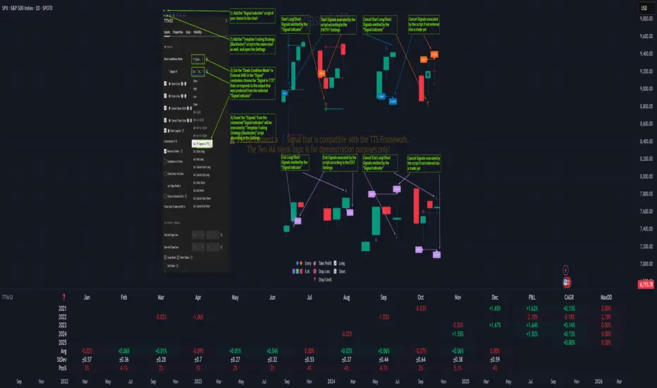
[FN] Strategy - Store Level on ConditionThis is a function that you can use in strategies. Not a strategy in and of itself.
Example thumbnail is showing the function applied to a strategy.
Oftentimes, I am asked a question regarding how to hold a variable at a specific, constant level over a conditional period of time. This question is always asked in a very long convoluted way like "I want the strategy to know what the high of the last pivot was while I'm in a long." or some other variation of wanting a script to remember something from prior bars.
This function is designed to store a price or some numeric level on the bar that your conditional (bool) statements determine that it should be stored. In this construct, you would set conditional statement(s) to flip the 'hold condition' to be true on the next bar, then hold that value until either the "hold condition" is no longer true or the initial conditions trigger again, causing an update to the level that you want to capture.
You still have to come up with the logic for the start condition and hold condition on your own, but I've provided an example that should give you an idea of how to accomplish this and customize/deploy the function for your purposes.
The function will return 'na' when neither the start condition nor hold condition are true. There's multiple ways to implement this and variations on how the level is chosen. I've written extensive notes in the script to guide you through the logic behind the function. My hope is that it will be useful to those trying to build strategies or anyone attempting to get their script to remember a level under given conditions.
In the thumbnail example, the take profit level is defined at the beginning of the trade and held until the take profit order executes. The order execution is a separate matter. However, storing the take-profit level at a static value is key to telling the strategy.exit() function what price to execute a limit exit order at.
Example: strategy.exit("Exit Long", from_entry = "long", qty_percent = 100, limit = stored_value)
Let me know how it works out for you and if I can be of any assistance.
Note: Strategy results are mainly derived from the fact that the strategy is long-only, the NQ only goes up, and there is no stop loss in place. So don't ask for the specific strategy, because unless you're trading a single contract with a $500,000 account, you'll probably get liquidated using this strategy as it is presented.

CCI 0Trend Strategy (by Marcoweb) v1.0Hi guys,
I am trying to create a strategy that consists in the crossover/under of the 0 line of the Commodity Channel Index . Every time the price crosses over the 0 line in the CCI the strategy has to long getting short on the cross under and viceversa.
I have published here another script strategy (consists in a crossover/under of the Overbought/Oversold levels of the CCI) that works so I could have the opportunity to share with you the main idea that as per now is mistaken:
//@version=2
strategy(title="CCI 0Trend Strategy (by Marcoweb) v1.0", shorttitle="CCI_0T_Stra_v1.0", overlay=true)
///////////// CCI
length = input(20, minval=1)
src = input(close, title="Source")
ma = sma(src, length)
cci = (src - ma) / (0.015 * dev(src, length))
plot(cci, color=black)
band1 = hline(100, color=blue, linestyle=solid)
band0 = hline(-100, color=red, linestyle=solid)
bandl = hline(0, color=orange, linestyle=solid)
fill(band1, band0, color=olive)
p1 = plot(band0, color=red,title="-100")
p2 = plot(band1, color=blue,title="100")
p3 = plot(bandl, color=orange,title="0")
///////////// CCI 0Trend Strategy (by Marcoweb) v1.0 Strategy
if (not na(cci))
if (crossover(cci, bandl)
strategy.entry("CCI_L", strategy.long, stop=bandl, oca_type=strategy.oca.cancel, comment="CCI_L")
else
strategy.cancel(id="CCI_L")
if (crossunder(cci, bandl)
strategy.entry("CCI_S", strategy.short, stop=bandl, oca_type=strategy.oca.cancel, comment="CCI_S")
else
strategy.cancel(id="CCI_S")
//plot(strategy.equity, title="equity", color=red, linewidth=2, style=areabr)
With this coding I get the error : line 24 (if (crossover(cci, bandl): mismatched input '|E|' expecting RPAR
Hope you like the idea ;)

NEXT GEN INSPIRED BY OLIVER VELEZDYOR NFA
1. Initial Setup & Application
Load the Strategy to your desired chart (e.g., EURUSD M5, as suggested by the script's backtest).
Overlay: Ensure the script is set to overlay=true (which it is) so the signals and Moving Averages plot directly on the price chart.
Equity Management: Review the initial strategy settings for capital and position sizing:
Initial Capital: Defaults to 10,000.
Default Qty Type: Set to strategy.percent_of_equity (22%), meaning 22% of your available equity is used per trade. Adjust this percentage based on your personal risk tolerance.
2. Reviewing Key Indicator Inputs
The script uses default values that are optimized, but you can adjust them in the settings panel:
Fast EMA: Defaults to 9 (e.g., a 9-period Exponential Moving Average).
Slow EMA: Defaults to 21 (e.g., a 21-period Exponential Moving Average). These EMAs define the short-term trend.
ATR: Defaults to 14 (Average True Range). Used to dynamically calculate volatility for SL/TP distances.
Final R:R: Defaults to 4.5 (minimum R:R required for a signal). This is the core of the strategy's high reward goal.
3. Interpreting Entry Signals
A trade signal is generated only when all conditions—EMA trend, "Elephant Logic" momentum, and non-ranging market—are met.
Long Signal: Appears as a green triangle (▲) below the bar, labeled "COMBO".
Short Signal: Appears as a red triangle (▼) above the bar, labeled "COMBO".
Live Plan: Upon signal, a detailed label is immediately plotted on the chart showing the FULL BATTLE PLAN:
SL: Calculated Stop Loss price.
TP: Calculated Take Profit price (based on the Final R:R).
Risk/Reward Pips: The calculated pips for the trade's risk and reward.
R:R = 1:4.5: The exact Risk-to-Reward ratio.
4. Understanding Market Conditions & Visuals
The script provides visuals to help you understand the current market state:
Trend EMAs: The 9 EMA (green) and 21 EMA (purple/magenta) are plotted to show the underlying trend.
Long trades only fire when Price > 9 EMA > 21 EMA.
Short trades only fire when Price < 9 EMA < 21 EMA.
Ranging Market (Rejection): Bars turn a light gray/silver when the proprietary "Reject Ranging" logic is active, indicating a low-volatility period. No new trades will be taken during these bars.
Momentum Bar: Bars turn a gold/yellow color when the "Elephant Logic" (high-momentum, large-body candles over 2-3 periods) is detected, highlighting powerful price movement.
5. Execution and Exit Logic
The strategy handles entry, scaling, and exit automatically:
Entry: A market order is placed (strategy.entry) immediately upon the bar where the longSetup or shortSetup condition is met.
Scaling Out (+1R): If the trade moves favorably by an amount equal to the initial risk (1R), the script closes a portion of the position (strategy.close with comment "+1R"). This partial exit locks in profit equivalent to the initial risk.
Re-entry (Pyramiding): After the +1R exit, the strategy attempts a re-entry (LONG RE/SHORT RE diamond plot) if the price meets certain criteria near the 9 EMA, trying to capitalize on further trend continuation.
Final Exits:
Take Profit: A limit order is set at the calculated TP level (stopDist * minRR).
Stop Loss: A stop order is set at the calculated SL level (stopDist * 1.3), slightly wider than the initial SL distance, likely to account for spread/slippage, ensuring the maximum loss is defined.
Trailing Stop: A trailing stop is applied to the re-entry positions (LONG RE/SHORT RE) to protect profits as the market moves further in the direction of the trade.

COT IndexTHE HIDDEN INTELLIGENCE IN FUTURES MARKETS
What if you could see what the smartest players in the futures markets are doing before the crowd catches on? While retail traders chase momentum indicators and moving averages, obsess over Japanese candlestick patterns, and debate whether the RSI should be set to fourteen or twenty-one periods, institutional players leave footprints in the sand through their mandatory reporting to the Commodity Futures Trading Commission. These footprints, published weekly in the Commitment of Traders reports, have been hiding in plain sight for decades, available to anyone with an internet connection, yet remarkably few traders understand how to interpret them correctly. The COT Index indicator transforms this raw institutional positioning data into actionable trading signals, bringing Wall Street intelligence to your trading screen without requiring expensive Bloomberg terminals or insider connections.
The uncomfortable truth is this: Most retail traders operate in a binary world. Long or short. Buy or sell. They apply technical analysis to individual positions, constrained by limited capital that forces them to concentrate risk in single directional bets. Meanwhile, institutional traders operate in an entirely different dimension. They manage portfolios dynamically weighted across multiple markets, adjusting exposure based on evolving market conditions, correlation shifts, and risk assessments that retail traders never see. A hedge fund might be simultaneously long gold, short oil, neutral on copper, and overweight agricultural commodities, with position sizes calibrated to volatility and portfolio Greeks. When they increase gold exposure from five percent to eight percent of portfolio allocation, this rebalancing decision reflects sophisticated analysis of opportunity cost, risk parity, and cross-market dynamics that no individual chart pattern can capture.
This portfolio reweighting activity, multiplied across hundreds of institutional participants, manifests in the aggregate positioning data published weekly by the CFTC. The Commitment of Traders report does not show individual trades or strategies. It shows the collective footprint of how actual commercial hedgers and large speculators have allocated their capital across different markets. When mining companies collectively increase forward gold sales to hedge thirty percent more production than last quarter, they are not reacting to a moving average crossover. They are making strategic allocation decisions based on production forecasts, cost structures, and price expectations derived from operational realities invisible to outside observers. This is portfolio management in action, revealed through positioning data rather than price charts.
If you want to understand how institutional capital actually flows, how sophisticated traders genuinely position themselves across market cycles, the COT report provides a rare window into that hidden world. But understand what you are getting into. This is not a tool for scalpers seeking confirmation of the next five-minute move. This is not an oscillator that flashes oversold at market bottoms with convenient precision. COT analysis operates on a timescale measured in weeks and months, revealing positioning shifts that precede major market turns but offer no precision timing. The data arrives three days stale, published only once per week, capturing strategic positioning rather than tactical entries.
If you need instant gratification, if you trade intraday moves, if you demand mechanical signals with ninety percent accuracy, close this document now. COT analysis rewards patience, position sizing discipline, and tolerance for being early. It punishes impatience, overleveraging, and the expectation that any single indicator can substitute for market understanding.
The premise is deceptively simple. Every Tuesday, large traders in futures markets must report their positions to the CFTC. By Friday afternoon, this data becomes public. Academic research spanning three decades has consistently shown that not all market participants are created equal. Some traders consistently profit while others consistently lose. Some anticipate major turning points while others chase trends into exhaustion. Bessembinder and Chan (1992) demonstrated in their seminal study that commercial hedgers, those with actual exposure to the underlying commodity or financial instrument, possess superior forecasting ability compared to speculators. Their research, published in the Journal of Finance, found statistically significant predictive power in commercial positioning, particularly at extreme levels. This finding challenged the efficient market hypothesis and opened the door to a new approach to market analysis based on positioning rather than price alone.
Think about what this means. Every week, the government publishes a report showing you exactly how the most informed market participants are positioned. Not their opinions. Not their predictions. Their actual money at risk. When agricultural producers collectively hold their largest short hedge in five years, they are not making idle speculation. They are locking in prices for crops they will harvest, informed by private knowledge of weather conditions, soil quality, inventory levels, and demand expectations invisible to outside observers. When energy companies aggressively hedge forward production at current prices, they reveal information about expected supply that no analyst report can capture. This is not technical analysis based on past prices. This is not fundamental analysis based on publicly available data. This is behavioral analysis based on how the smartest money is actually positioned, how institutions allocate capital across portfolios, and how those allocation decisions shift as market conditions evolve.
WHY SOME TRADERS KNOW MORE THAN OTHERS
Building on this foundation, Sanders, Boris and Manfredo (2004) conducted extensive research examining the behaviour patterns of different trader categories. Their work, which analyzed over a decade of COT data across multiple commodity markets, revealed a fascinating dynamic that challenges much of what retail traders are taught. Commercial hedgers consistently positioned themselves against market extremes, buying when speculators were most bearish and selling when speculators reached peak bullishness. The contrarian positioning of commercials was not random noise but rather reflected their superior information about supply and demand fundamentals. Meanwhile, large speculators, primarily hedge funds and commodity trading advisors, exhibited strong trend-following behaviour that often amplified market moves beyond fundamental values. Small traders, the retail participants, consistently entered positions late in trends, frequently near turning points, making them reliable contrary indicators.
Wang (2003) extended this research by demonstrating that the predictive power of commercial positioning varies significantly across different commodity sectors. His analysis of agricultural commodities showed particularly strong forecasting ability, with commercial net positions explaining up to fifteen percent of return variance in subsequent weeks. This finding suggests that the informational advantages of hedgers are most pronounced in markets where physical supply and demand fundamentals dominate, as opposed to purely financial markets where information asymmetries are smaller. When a corn farmer hedges six months of expected harvest, that decision incorporates private observations about rainfall patterns, crop health, pest pressure, and local storage capacity that no distant analyst can match. When an oil refinery hedges crude oil purchases and gasoline sales simultaneously, the spread relationships reveal expectations about refining margins that reflect operational realities invisible in public data.
The theoretical mechanism underlying these empirical patterns relates to information asymmetry and different participant motivations. Commercial hedgers engage in futures markets not for speculative profit but to manage business risks. An agricultural producer selling forward six months of expected harvest is not making a bet on price direction but rather locking in revenue to facilitate financial planning and ensure business viability. However, this hedging activity necessarily incorporates private information about expected supply, inventory levels, weather conditions, and demand trends that the hedger observes through their commercial operations (Irwin and Sanders, 2012). When aggregated across many participants, this private information manifests in collective positioning.
Consider a gold mining company deciding how much forward production to hedge. Management must estimate ore grades, recovery rates, production costs, equipment reliability, labor availability, and dozens of other operational variables that determine whether locking in prices at current levels makes business sense. If the industry collectively hedges more aggressively than usual, it suggests either exceptional production expectations or concern about sustaining current price levels or combination of both. Either way, this positioning reveals information unavailable to speculators analyzing price charts and economic data. The hedger sees the physical reality behind the financial abstraction.
Large speculators operate under entirely different incentives and constraints. Commodity Trading Advisors managing billions in assets typically employ systematic, trend-following strategies that respond to price momentum rather than fundamental supply and demand. When crude oil rallies from sixty dollars to seventy dollars per barrel, these systems generate buy signals. As the rally continues to eighty dollars, position sizes increase. The strategy works brilliantly during sustained trends but becomes a liability at reversals. By the time oil reaches ninety dollars, trend-following funds are maximally long, having accumulated positions progressively throughout the rally. At this point, they represent not smart money anticipating further gains but rather crowded money vulnerable to reversal. Sanders, Boris and Manfredo (2004) documented this pattern across multiple energy markets, showing that extreme speculator positioning typically marked late-stage trend exhaustion rather than early-stage trend development.
Small traders, the retail participants who fall below reporting thresholds, display the weakest forecasting ability. Wang (2003) found that small trader positioning exhibited negative correlation with subsequent returns, meaning their aggregate positioning served as a reliable contrary indicator. The explanation combines several factors. Retail traders often lack the capital reserves to weather normal market volatility, leading to premature exits from positions that would eventually prove profitable. They tend to receive information through slower channels, entering trends after mainstream media coverage when institutional participants are preparing to exit. Perhaps most importantly, they trade with emotion, buying into euphoria and selling into panic at precisely the wrong times.
At major turning points, the three groups often position opposite each other with commercials extremely bearish, large speculators extremely bullish, and small traders piling into longs at the last moment. These high-divergence environments frequently precede increased volatility and trend reversals. The insiders with business exposure quietly exit as the momentum traders hit maximum capacity and retail enthusiasm peaks. Within weeks, the reversal begins, and positions unwind in the opposite sequence.
FROM RAW DATA TO ACTIONABLE SIGNALS
The COT Index indicator operationalizes these academic findings into a practical trading tool accessible through TradingView. At its core, the indicator normalizes net positioning data onto a zero to one hundred scale, creating what we call the COT Index. This normalization is critical because absolute position sizes vary dramatically across different futures contracts and over time. A commercial trader holding fifty thousand contracts net long in crude oil might be extremely bullish by historical standards, or it might be quite neutral depending on the context of total market size and historical ranges. Raw position numbers mean nothing without context. The COT Index solves this problem by calculating where current positioning stands relative to its range over a specified lookback period, typically two hundred fifty-two weeks or approximately five years of weekly data.
The mathematical transformation follows the methodology originally popularized by legendary trader Larry Williams, though the underlying concept appears in statistical normalization techniques across many fields. For any given trader category, we calculate the highest and lowest net position values over the lookback period, establishing the historical range for that specific market and trader group. Current positioning is then expressed as a percentage of this range, where zero represents the most bearish positioning ever seen in the lookback window and one hundred represents the most bullish extreme. A reading of fifty indicates positioning exactly in the middle of the historical range, suggesting neither extreme optimism nor pessimism relative to recent history (Williams and Noseworthy, 2009).
This index-based approach allows for meaningful comparison across different markets and time periods, overcoming the scaling problems inherent in analyzing raw position data. A commercial index reading of eighty-five in gold carries the same interpretive meaning as an eighty-five reading in wheat or crude oil, even though the absolute position sizes differ by orders of magnitude. This standardization enables systematic analysis across entire futures portfolios rather than requiring market-specific expertise for each contract.
The lookback period selection involves a fundamental tradeoff between responsiveness and stability. Shorter lookback periods, perhaps one hundred twenty-six weeks or approximately two and a half years, make the index more sensitive to recent positioning changes. However, it also increases noise and produces more false signals. Longer lookback periods, perhaps five hundred weeks or approximately ten years, create smoother readings that filter short-term noise but become slower to recognize regime changes. The indicator settings allow users to adjust this parameter based on their trading timeframe, risk tolerance, and market characteristics.
UNDERSTANDING CFTC DATA STRUCTURES
The indicator supports both Legacy and Disaggregated COT report formats, reflecting the evolution of CFTC reporting standards over decades of market development. Legacy reports categorize market participants into three broad groups: commercial traders (hedgers with underlying business exposure), non-commercial traders (large speculators seeking profit without commercial interest), and non-reportable traders (small speculators below reporting thresholds). Each category brings distinct motivations and information advantages to the market (CFTC, 2020).
The Disaggregated reports, introduced in September 2009 for physical commodity markets, provide finer granularity by splitting participants into five categories (CFTC, 2009). Producer and merchant positions capture those actually producing, processing, or merchandising the physical commodity. Swap dealers represent financial intermediaries facilitating derivative transactions for clients. Managed money includes commodity trading advisors and hedge funds executing systematic or discretionary strategies. Other reportables encompasses diverse participants not fitting the main categories. Small traders remain as the fifth group, representing retail participation.
This enhanced categorization reveals nuances invisible in Legacy reports, particularly distinguishing between different types of institutional capital and their distinct behavioural patterns. The indicator automatically detects which report type is appropriate for each futures contract and adjusts the display accordingly.
Importantly, Disaggregated reports exist only for physical commodity futures. Agricultural commodities like corn, wheat, and soybeans have Disaggregated reports because clear producer, merchant, and swap dealer categories exist. Energy commodities like crude oil and natural gas similarly have well-defined commercial hedger categories. Metals including gold, silver, and copper also receive Disaggregated treatment (CFTC, 2009). However, financial futures such as equity index futures, Treasury bond futures, and currency futures remain available only in Legacy format. The CFTC has indicated no plans to extend Disaggregated reporting to financial futures due to different market structures and participant categories in these instruments (CFTC, 2020).
THE BEHAVIORAL FOUNDATION
Understanding which trader perspective to follow requires appreciation of their distinct trading styles, success rates, and psychological profiles. Commercial hedgers exhibit anticyclical behaviour rooted in their fundamental knowledge and business imperatives. When agricultural producers hedge forward sales during harvest season, they are not speculating on price direction but rather locking in revenue for crops they will harvest. Their business requires converting volatile commodity exposure into predictable cash flows to facilitate planning and ensure survival through difficult periods. Yet their aggregate positioning reveals valuable information because these hedging decisions incorporate private information about supply conditions, inventory levels, weather observations, and demand expectations that hedgers observe through their commercial operations (Bessembinder and Chan, 1992).
Consider a practical example from energy markets. Major oil companies continuously hedge portions of forward production based on price levels, operational costs, and financial planning needs. When crude oil trades at ninety dollars per barrel, they might aggressively hedge the next twelve months of production, locking in prices that provide comfortable profit margins above their extraction costs. This hedging appears as short positioning in COT reports. If oil rallies further to one hundred dollars, they hedge even more aggressively, viewing these prices as exceptional opportunities to secure revenue. Their short positioning grows increasingly extreme. To an outside observer watching only price charts, the rally suggests bullishness. But the commercial positioning reveals that the actual producers of oil find these prices attractive enough to lock in years of sales, suggesting skepticism about sustaining even higher levels. When the eventual reversal occurs and oil declines back to eighty dollars, the commercials who hedged at ninety and one hundred dollars profit while speculators who chased the rally suffer losses.
Large speculators or managed money traders operate under entirely different incentives and constraints. Their systematic, momentum-driven strategies mean they amplify existing trends rather than anticipate reversals. Trend-following systems, the most common approach among large speculators, by definition require confirmation of trend through price momentum before entering positions (Sanders, Boris and Manfredo, 2004). When crude oil rallies from sixty dollars to eighty dollars per barrel over several months, trend-following algorithms generate buy signals based on moving average crossovers, breakouts, and other momentum indicators. As the rally continues, position sizes increase according to the systematic rules.
However, this approach becomes a liability at turning points. By the time oil reaches ninety dollars after a sustained rally, trend-following funds are maximally long, having accumulated positions progressively throughout the move. At this point, their positioning does not predict continued strength. Rather, it often marks late-stage trend exhaustion. The psychological and mechanical explanation is straightforward. Trend followers by definition chase price momentum, entering positions after trends establish rather than anticipating them. Eventually, they become fully invested just as the trend nears completion, leaving no incremental buying power to sustain the rally. When the first signs of reversal appear, systematic stops trigger, creating a cascade of selling that accelerates the downturn.
Small traders consistently display the weakest track record across academic studies. Wang (2003) found that small trader positioning exhibited negative correlation with subsequent returns in his analysis across multiple commodity markets. This result means that whatever small traders collectively do, the opposite typically proves profitable. The explanation for small trader underperformance combines several factors documented in behavioral finance literature. Retail traders often lack the capital reserves to weather normal market volatility, leading to premature exits from positions that would eventually prove profitable. They tend to receive information through slower channels, learning about commodity trends through mainstream media coverage that arrives after institutional participants have already positioned. Perhaps most importantly, retail traders are more susceptible to emotional decision-making, buying into euphoria and selling into panic at precisely the wrong times (Tharp, 2008).
SETTINGS, THRESHOLDS, AND SIGNAL GENERATION
The practical implementation of the COT Index requires understanding several key features and settings that users can adjust to match their trading style, timeframe, and risk tolerance. The lookback period determines the time window for calculating historical ranges. The default setting of two hundred fifty-two bars represents approximately one year on daily charts or five years on weekly charts, balancing responsiveness with stability. Conservative traders seeking only the most extreme, highest-probability signals might extend the lookback to five hundred bars or more. Aggressive traders seeking earlier entry and willing to accept more false positives might reduce it to one hundred twenty-six bars or even less for shorter-term applications.
The bullish and bearish thresholds define signal generation levels. Default settings of eighty and twenty respectively reflect academic research suggesting meaningful information content at these extremes. Readings above eighty indicate positioning in the top quintile of the historical range, representing genuine extremes rather than temporary fluctuations. Conversely, readings below twenty occupy the bottom quintile, indicating unusually bearish positioning (Briese, 2008).
However, traders must recognize that appropriate thresholds vary by market, trader category, and personal risk tolerance. Some futures markets exhibit wider positioning swings than others due to seasonal patterns, volatility characteristics, or participant behavior. Conservative traders seeking high-probability setups with fewer signals might raise thresholds to eighty-five and fifteen. Aggressive traders willing to accept more false positives for earlier entry could lower them to seventy-five and twenty-five.
The key is maintaining meaningful differentiation between bullish, neutral, and bearish zones. The default settings of eighty and twenty create a clear three-zone structure. Readings from zero to twenty represent bearish territory where the selected trader group holds unusually bearish positions. Readings from twenty to eighty represent neutral territory where positioning falls within normal historical ranges. Readings from eighty to one hundred represent bullish territory where the selected trader group holds unusually bullish positions.
The trading perspective selection determines which participant group the indicator follows, fundamentally shaping interpretation and signal meaning. For counter-trend traders seeking reversal opportunities, monitoring commercial positioning makes intuitive sense based on the academic research discussed earlier. When commercials reach extreme bearish readings below twenty, indicating unprecedented short positioning relative to recent history, they are effectively betting against the crowd. Given their informational advantages demonstrated by Bessembinder and Chan (1992), this contrarian stance often precedes major bottoms.
Trend followers might instead monitor large speculator positioning, but with inverted logic compared to commercials. When managed money reaches extreme bullish readings above eighty, the trend may be exhausting rather than accelerating. This seeming paradox reflects their late-cycle participation documented by Sanders, Boris and Manfredo (2004). Sophisticated traders thus use speculator extremes as fade signals, entering positions opposite to speculator consensus.
Small trader monitoring serves primarily as a contrary indicator for all trading styles. Extreme small trader bullishness above seventy-five or eighty typically warns of retail FOMO at market tops. Extreme small trader bearishness below twenty or twenty-five often marks capitulation bottoms where the last weak hands have sold.
VISUALIZATION AND USER INTERFACE
The visual design incorporates multiple elements working together to facilitate decision-making and maintain situational awareness during active trading. The primary COT Index line plots in bold with adjustable line width, defaulting to two pixels for clear visibility against busy price charts. An optional glow effect, controlled by a simple toggle, adds additional visual prominence through multiple plot layers with progressively increasing transparency and width.
A twenty-one period exponential moving average overlays the index line, providing trend context for positioning changes. When the index crosses above its moving average, it signals accelerating bullish sentiment among the selected trader group regardless of whether absolute positioning is extreme. Conversely, when the index crosses below its moving average, it signals deteriorating sentiment and potentially the beginning of a reversal in positioning trends.
The EMA provides a dynamic reference line for assessing positioning momentum. When the index trades far above its EMA, positioning is not only extreme in absolute terms but also building with momentum. When the index trades far below its EMA, positioning is contracting or reversing, which may indicate weakening conviction even if absolute levels remain elevated.
The data table positioned at the top right of the chart displays eleven metrics for each trader category, transforming the indicator from a simple index calculation into an analytical dashboard providing multidimensional market intelligence. Beyond the COT Index itself, users can monitor positioning extremity, which measures how unusual current levels are compared to historical norms using statistical techniques. The extremity metric clarifies whether a reading represents the ninety-fifth or ninety-ninth percentile, with values above two standard deviations indicating genuinely exceptional positioning.
Market power quantifies each group's influence on total open interest. This metric expresses each trader category's net position as a percentage of total market open interest. A commercial entity holding forty percent of total open interest commands significantly more influence than one holding five percent, making their positioning signals more meaningful.
Momentum and rate of change metrics reveal whether positions are building or contracting, providing early warning of potential regime shifts. Position velocity measures the rate of change in positioning changes, effectively a second derivative providing even earlier insight into inflection points.
Sentiment divergence highlights disagreements between commercial and speculative positioning. This metric calculates the absolute difference between normalized commercial and large speculator index values. Wang (2003) found that these high-divergence environments frequently preceded increased volatility and reversals.
The table also displays concentration metrics when available, showing how positioning is distributed among the largest handful of traders in each category. High concentration indicates a few dominant players controlling most of the positioning, while low concentration suggests broad-based participation across many traders.
THE ALERT SYSTEM AND MONITORING
The alert system, comprising five distinct alert conditions, enables systematic monitoring of dozens of futures markets without constant screen watching. The bullish and bearish COT signal alerts trigger when the index crosses user-defined thresholds, indicating the selected trader group has reached extreme positioning worthy of attention. These alerts fire in real-time as new weekly COT data publishes, typically Friday afternoon following the Tuesday measurement date.
Extreme positioning alerts fire at ninety and ten index levels, representing the top and bottom ten percent of the historical range, warning of particularly stretched readings that historically precede reversals with high probability. When commercials reach a COT Index reading below ten, they are expressing their most bearish stance in the entire lookback period.
The data staleness alert notifies users when COT reports have not updated for more than ten days, preventing reliance on outdated information for trading decisions. Government shutdowns or federal holidays can interrupt the normal Friday publication schedule. Using stale signals while believing them current creates dangerous false confidence.
The indicator's watermark information display positioned in the bottom right corner provides essential context at a glance. This persistent display shows the symbol and timeframe, the COT report date timestamp, days since last update, and the current signal state. A trader analyzing a potential short entry in crude oil can glance at the watermark to instantly confirm positioning context without interrupting analysis flow.
LIMITATIONS AND REALISTIC EXPECTATIONS
Practical application requires understanding both the indicator's considerable strengths and inherent limitations. COT data inherently lags price action by three days, as Tuesday positions are not published until Friday afternoon. This delay means the indicator cannot catch rapid intraday reversals or respond to surprise news events. Traders using the COT Index for timing entries must accept this latency and focus on swing trading and position trading timeframes where three-day lags matter less than in day trading or scalping.
The weekly publication schedule similarly makes the indicator unsuitable for short-term trading strategies requiring immediate feedback. The COT Index works best for traders operating on weekly or longer timeframes, where positioning shifts measured in weeks and months align with trading horizon.
Extreme COT readings can persist far longer than typical technical indicators suggest, testing the patience and capital reserves of traders attempting to fade them. When crude oil enters a sustained bull market driven by genuine supply disruptions, commercial hedgers may maintain bearish positioning for many months as prices grind higher. A commercial COT Index reading of fifteen indicating extreme bearishness might persist for three months while prices continue rallying before finally reversing. Traders without sufficient capital and risk tolerance to weather such drawdowns will exit prematurely, precisely when the signal is about to work (Irwin and Sanders, 2012).
Position sizing discipline becomes paramount when implementing COT-based strategies. Rather than risking large percentages of capital on individual signals, successful COT traders typically allocate modest position sizes across multiple signals, allowing some to take time to mature while others work more quickly.
The indicator also cannot overcome fundamental regime changes that alter the structural drivers of markets. If gold enters a true secular bull market driven by monetary debasement, commercial hedgers may remain persistently bearish as mining companies sell forward years of production at what they perceive as favorable prices. Their positioning indicates valuation concerns from a production cost perspective, but cannot stop prices from rising if investment demand overwhelms physical supply-demand balance.
Similarly, structural changes in market participation can alter the meaning of positioning extremes. The growth of commodity index investing in the two thousands brought massive passive long-only capital into futures markets, fundamentally changing typical positioning ranges. Traders relying on COT signals without recognizing this regime change would have generated numerous false bearish signals during the commodity supercycle from 2003 to 2008.
The research foundation supporting COT analysis derives primarily from commodity markets where the commercial hedger information advantage is most pronounced. Studies specifically examining financial futures like equity indices and bonds show weaker but still present effects. Traders should calibrate expectations accordingly, recognizing that COT analysis likely works better for crude oil, natural gas, corn, and wheat than for the S&P 500, Treasury bonds, or currency futures.
Another important limitation involves the reporting threshold structure. Not all market participants appear in COT data, only those holding positions above specified minimums. In markets dominated by a few large players, concentration metrics become critical for proper interpretation. A single large trader accounting for thirty percent of commercial positioning might skew the entire category if their individual circumstances are idiosyncratic rather than representative.
GOLD FUTURES DURING A HYPOTHETICAL MARKET CYCLE
Consider a practical example using gold futures during a hypothetical but realistic market scenario that illustrates how the COT Index indicator guides trading decisions through a complete market cycle. Suppose gold has rallied from fifteen hundred to nineteen hundred dollars per ounce over six months, driven by inflation concerns following aggressive monetary expansion, geopolitical uncertainty, and sustained buying by Asian central banks for reserve diversification.
Large speculators, operating primarily trend-following strategies, have accumulated increasingly bullish positions throughout this rally. Their COT Index has climbed progressively from forty-five to eighty-five. The table display shows that large speculators now hold net long positions representing thirty-two percent of total open interest, their highest in four years. Momentum indicators show positive readings, indicating positions are still building though at a decelerating rate. Position velocity has turned negative, suggesting the pace of position building is slowing.
Meanwhile, commercial hedgers have responded to the rally by aggressively selling forward production and inventory. Their COT Index has moved inversely to price, declining from fifty-five to twenty. This bearish commercial positioning represents mining companies locking in forward sales at prices they view as attractive relative to production costs. The table shows commercials now hold net short positions representing twenty-nine percent of total open interest, their most bearish stance in five years. Concentration metrics indicate this positioning is broadly distributed across many commercial entities, suggesting the bearish stance reflects collective industry view rather than idiosyncratic positioning by a single firm.
Small traders, attracted by mainstream financial media coverage of gold's impressive rally, have recently piled into long positions. Their COT Index has jumped from forty-five to seventy-eight as retail investors chase the trend. Television financial networks feature frequent segments on gold with bullish guests. Internet forums and social media show surging retail interest. This retail enthusiasm historically marks late-stage trend development rather than early opportunity.
The COT Index indicator, configured to monitor commercial positioning from a contrarian perspective, displays a clear bearish signal given the extreme commercial short positioning. The table displays multiple confirming metrics: positioning extremity shows commercials at the ninety-sixth percentile of bearishness, market power indicates they control twenty-nine percent of open interest, and sentiment divergence registers sixty-five, indicating massive disagreement between commercial hedgers and large speculators. This divergence, the highest in three years, places the market in the historically high-risk category for reversals.
The interpretation requires nuance and consideration of context beyond just COT data. Commercials are not necessarily predicting an imminent crash. Rather, they are hedging business operations at what they collectively view as favorable price levels. However, the data reveals they have sold unusually large quantities of forward production, suggesting either exceptional production expectations for the year ahead or concern about sustaining current price levels or combination of both. Combined with extreme speculator positioning indicating a crowded long trade, and small trader enthusiasm confirming retail FOMO, the confluence suggests elevated reversal risk even if the precise timing remains uncertain.
A prudent trader analyzing this situation might take several actions based on COT Index signals. Existing long positions could be tightened with closer stop losses. Profit-taking on a portion of long exposure could lock in gains while maintaining some participation. Some traders might initiate modest short positions as portfolio hedges, sizing them appropriately for the inherent uncertainty in timing reversals. Others might simply move to the sidelines, avoiding new long entries until positioning normalizes.
The key lesson from case study analysis is that COT signals provide probabilistic edges rather than deterministic predictions. They work over many observations by identifying higher-probability configurations, not by generating perfect calls on individual trades. A fifty-five percent win rate with proper risk management produces substantial profits over time, yet still means forty-five percent of signals will be premature or wrong. Traders must embrace this probabilistic reality rather than seeking the impossible goal of perfect accuracy.
INTEGRATION WITH TRADING SYSTEMS
Integration with existing trading systems represents a natural and powerful use case for COT analysis, adding a positioning dimension to price-based technical approaches or fundamental analytical frameworks. Few traders rely exclusively on a single indicator or methodology. Rather, they build systems that synthesize multiple information sources, with each component addressing different aspects of market behavior.
Trend followers might use COT extremes as regime filters, modifying position sizing or avoiding new trend entries when positioning reaches levels historically associated with reversals. Consider a classic trend-following system based on moving average crossovers and momentum breakouts. Integration of COT analysis adds nuance. When large speculator positioning exceeds ninety or commercial positioning falls below ten, the regime filter recognizes elevated reversal risk. The system might reduce position sizing by fifty percent for new signals during these high-risk periods (Kaufman, 2013).
Mean reversion traders might require COT signal confluence before fading extended moves. When crude oil becomes technically overbought and large speculators show extreme long positioning above eighty-five, both signals confirm. If only technical indicators show extremes while positioning remains neutral, the potential short signal is rejected, avoiding fades of trends with underlying institutional support (Kaufman, 2013).
Discretionary traders can monitor the indicator as a continuous awareness tool, informing bias and position sizing without dictating mechanical entries and exits. A discretionary trader might notice commercial positioning shifting from neutral to progressively more bullish over several months. This trend informs growing positive bias even without triggering mechanical signals.
Multi-timeframe analysis represents another powerful integration approach. A trader might use daily charts for trade execution and timing while monitoring weekly COT positioning for strategic context. When both timeframes align, highest-probability opportunities emerge.
Portfolio construction for futures traders can incorporate COT signals as an additional selection criterion. Markets showing strong technical setups AND favorable COT positioning receive highest allocations. Markets with strong technicals but neutral or unfavorable positioning receive reduced allocations.
ADVANCED METRICS AND INTERPRETATION
The metrics table transforms simple positioning data into multidimensional market intelligence. Position extremity, calculated as the absolute deviation from the historical mean normalized by standard deviation, helps identify truly unusual readings versus routine fluctuations. A reading above two standard deviations indicates ninety-fifth percentile or higher extremity. Above three standard deviations indicates ninety-ninth percentile or higher, genuinely rare positioning that historically precedes major events with high probability.
Market power, expressed as a percentage of total open interest, reveals whose positioning matters most from a mechanical market impact perspective. Consider two scenarios in gold futures. In scenario one, commercials show a COT Index reading of fifteen while their market power metric shows they hold net shorts representing thirty-five percent of open interest. This is a high-confidence bearish signal. In scenario two, commercials also show a reading of fifteen, but market power shows only eight percent. While positioning is extreme relative to this category's normal range, their limited market share means less mechanical influence on price.
The rate of change and momentum metrics highlight whether positions are accelerating or decelerating, often providing earlier warnings than absolute levels alone. A COT Index reading of seventy-five with rapidly building momentum suggests continued movement toward extremes. Conversely, a reading of eighty-five with decelerating or negative momentum indicates the positioning trend is exhausting.
Position velocity measures the rate of change in positioning changes, effectively a second derivative. When velocity shifts from positive to negative, it indicates that while positioning may still be growing, the pace of growth is slowing. This deceleration often precedes actual reversal in positioning direction by several weeks.
Sentiment divergence calculates the absolute difference between normalized commercial and large speculator index values. When commercials show extreme bearish positioning at twenty while large speculators show extreme bullish positioning at eighty, the divergence reaches sixty, representing near-maximum disagreement. Wang (2003) found that these high-divergence environments frequently preceded increased volatility and reversals. The mechanism is intuitive. Extreme divergence indicates the informed hedgers and momentum-following speculators have positioned opposite each other with conviction. One group will prove correct and profit while the other proves incorrect and suffers losses. The resolution of this disagreement through price movement often involves volatility.
The table also displays concentration metrics when available. High concentration indicates a few dominant players controlling most of the positioning within a category, while low concentration suggests broad-based participation. Broad-based positioning more reliably reflects collective market intelligence and industry consensus. If mining companies globally all independently decide to hedge aggressively at similar price levels, it suggests genuine industry-wide view about price valuations rather than circumstances specific to one firm.
DATA QUALITY AND RELIABILITY
The CFTC has maintained COT reporting in various forms since the nineteen twenties, providing nearly a century of positioning data across multiple market cycles. However, data quality and reporting standards have evolved substantially over this long period. Modern electronic reporting implemented in the late nineteen nineties and early two thousands significantly improved accuracy and timeliness compared to earlier paper-based systems.
Traders should understand that COT reports capture positions as of Tuesday's close each week. Markets remain open three additional days before publication on Friday afternoon, meaning the reported data is three days stale when received. During periods of rapid market movement or major news events, this lag can be significant. The indicator addresses this limitation by including timestamp information and staleness warnings.
The three-day lag creates particular challenges during extreme volatility episodes. Flash crashes, surprise central bank interventions, geopolitical shocks, and other high-impact events can completely transform market positioning within hours. Traders must exercise judgment about whether reported positioning remains relevant given intervening events.
Reporting thresholds also mean that not all market participants appear in disaggregated COT data. Traders holding positions below specified minimums aggregate into the non-reportable or small trader category. This aggregation affects different markets differently. In highly liquid contracts like crude oil with thousands of participants, reportable traders might represent seventy to eighty percent of open interest. In thinly traded contracts with only dozens of active participants, a few large reportable positions might represent ninety-five percent of open interest.
Another data quality consideration involves trader classification into categories. The CFTC assigns traders to commercial or non-commercial categories based on reported business purpose and activities. However, this process is not perfect. Some entities engage in both commercial and speculative activities, creating ambiguity about proper classification. The transition to Disaggregated reports attempted to address some of these ambiguities by creating more granular categories.
COMPARISON WITH ALTERNATIVE APPROACHES
Several alternative approaches to COT analysis exist in the trading community beyond the normalization methodology employed by this indicator. Some analysts focus on absolute position changes week-over-week rather than index-based normalization. This approach calculates the change in net positioning from one week to the next. The emphasis falls on momentum in positioning changes rather than absolute levels relative to history. This method potentially identifies regime shifts earlier but sacrifices cross-market comparability (Briese, 2008).
Other practitioners employ more complex statistical transformations including percentile rankings, z-score standardization, and machine learning classification algorithms. Ruan and Zhang (2018) demonstrated that machine learning models applied to COT data could achieve modest improvements in forecasting accuracy compared to simple threshold-based approaches. However, these gains came at the cost of interpretability and implementation complexity.
The COT Index indicator intentionally employs a relatively straightforward normalization methodology for several important reasons. First, transparency enhances user understanding and trust. Traders can verify calculations manually and develop intuitive feel for what different readings mean. Second, academic research suggests that most of the predictive power in COT data comes from extreme positioning levels rather than subtle patterns requiring complex statistical methods to detect. Third, robust methods that work consistently across many markets and time periods tend to be simpler rather than more complex, reducing the risk of overfitting to historical data. Fourth, the complexity costs of implementation matter for retail traders without programming teams or computational infrastructure.
PSYCHOLOGICAL ASPECTS OF COT TRADING
Trading based on COT data requires psychological fortitude that differs from momentum-based approaches. Contrarian positioning signals inherently mean betting against prevailing market sentiment and recent price action. When commercials reach extreme bearish positioning, prices have typically been rising, sometimes for extended periods. The price chart looks bullish, momentum indicators confirm strength, moving averages align positively. The COT signal says bet against all of this. This psychological difficulty explains why COT analysis remains underutilized relative to trend-following methods.
Human psychology strongly predisposes us toward extrapolation and recency bias. When prices rally for months, our pattern-matching brains naturally expect continued rally. The recent price action dominates our perception, overwhelming rational analysis about positioning extremes and historical probabilities. The COT signal asking us to sell requires overriding these powerful psychological impulses.
The indicator design attempts to support the required psychological discipline through several features. Clear threshold markers and signal states reduce ambiguity about when signals trigger. When the commercial index crosses below twenty, the signal is explicit and unambiguous. The background shifts to red, the signal label displays bearish, and alerts fire. This explicitness helps traders act on signals rather than waiting for additional confirmation that may never arrive.
The metrics table provides analytical justification for contrarian positions, helping traders maintain conviction during inevitable periods of adverse price movement. When a trader enters short positions based on extreme commercial bearish positioning but prices continue rallying for several weeks, doubt naturally emerges. The table display provides reassurance. Commercial positioning remains extremely bearish. Divergence remains high. The positioning thesis remains intact even though price action has not yet confirmed.
Alert functionality ensures traders do not miss signals due to inattention while also not requiring constant monitoring that can lead to emotional decision-making. Setting alerts for COT extremes enables a healthier relationship with markets. When meaningful signals occur, alerts notify them. They can then calmly assess the situation and execute planned responses.
However, no indicator design can completely overcome the psychological difficulty of contrarian trading. Some traders simply cannot maintain short positions while prices rally. For these traders, COT analysis might be better employed as an exit signal for long positions rather than an entry signal for shorts.
Ultimately, successful COT trading requires developing comfort with probabilistic thinking rather than certainty-seeking. The signals work over many observations by identifying higher-probability configurations, not by generating perfect calls on individual trades. A fifty-five or sixty percent win rate with proper risk management produces substantial profits over years, yet still means forty to forty-five percent of signals will be premature or wrong. COT analysis provides genuine edge, but edge means probability advantage, not elimination of losing trades.
EDUCATIONAL RESOURCES AND CONTINUOUS LEARNING
The indicator provides extensive built-in educational resources through its documentation, detailed tooltips, and transparent calculations. However, mastering COT analysis requires study beyond any single tool or resource. Several excellent resources provide valuable extensions of the concepts covered in this guide.
Books and practitioner-focused monographs offer accessible entry points. Stephen Briese published The Commitments of Traders Bible in two thousand eight, offering detailed breakdowns of how different markets and trader categories behave (Briese, 2008). Briese's work stands out for its empirical focus and market-specific insights. Jack Schwager includes discussion of COT analysis within the broader context of market behavior in his book Market Sense and Nonsense (Schwager, 2012). Perry Kaufman's Trading Systems and Methods represents perhaps the most rigorous practitioner-focused text on systematic trading approaches including COT analysis (Kaufman, 2013).
Academic journal articles provide the rigorous statistical foundation underlying COT analysis. The Journal of Futures Markets regularly publishes research on positioning data and its predictive properties. Bessembinder and Chan's earlier work on systematic risk, hedging pressure, and risk premiums in futures markets provides theoretical foundation (Bessembinder, 1992). Chang's examination of speculator returns provides historical context (Chang, 1985). Irwin and Sanders provide essential skeptical perspective in their two thousand twelve article (Irwin and Sanders, 2012). Wang's two thousand three article provides one of the most empirical analyses of COT data across multiple commodity markets (Wang, 2003).
Online resources extend beyond academic and book-length treatments. The CFTC website provides free access to current and historical COT reports in multiple formats. The explanatory materials section offers detailed documentation of report construction, category definitions, and historical methodology changes. Traders serious about COT analysis should read these official CFTC documents to understand exactly what they are analyzing.
Commercial COT data services such as Barchart provide enhanced visualization and analysis tools beyond raw CFTC data. TradingView's educational materials, published scripts library, and user community provide additional resources for exploring different approaches to COT analysis.
The key to mastering COT analysis lies not in finding a single definitive source but rather in building understanding through multiple perspectives and information sources. Academic research provides rigorous empirical foundation. Practitioner-focused books offer practical implementation insights. Direct engagement with data through systematic backtesting develops intuition about how positioning dynamics manifest across different market conditions.
SYNTHESIZING KNOWLEDGE INTO PRACTICE
The COT Index indicator represents the synthesis of academic research, trading experience, and software engineering into a practical tool accessible to retail traders equipped with nothing more than a TradingView account and willingness to learn. What once required expensive data subscriptions, custom programming capabilities, statistical software, and institutional resources now appears as a straightforward indicator requiring only basic parameter selection and modest study to understand. This democratization of institutional-grade analysis tools represents a broader trend in financial markets over recent decades.
Yet technology and data access alone provide no edge without understanding and discipline. Markets remain relentlessly efficient at eliminating edges that become too widely known and mechanically exploited. The COT Index indicator succeeds only when users invest time learning the underlying concepts, understand the limitations and probability distributions involved, and integrate signals thoughtfully into trading plans rather than applying them mechanically.
The academic research demonstrates conclusively that institutional positioning contains genuine information about future price movements, particularly at extremes where commercial hedgers are maximally bearish or bullish relative to historical norms. This informational content is neither perfect nor deterministic but rather probabilistic, providing edge over many observations through identification of higher-probability configurations. Bessembinder and Chan's finding that commercial positioning explained modest but significant variance in future returns illustrates this probabilistic nature perfectly (Bessembinder and Chan, 1992). The effect is real and statistically significant, yet it explains perhaps ten to fifteen percent of return variance rather than most variance. Much of price movement remains unpredictable even with positioning intelligence.
The practical implication is that COT analysis works best as one component of a trading system rather than a standalone oracle. It provides the positioning dimension, revealing where the smart money has positioned and where the crowd has followed, but price action analysis provides the timing dimension. Fundamental analysis provides the catalyst dimension. Risk management provides the survival dimension. These components work together synergistically.
The indicator's design philosophy prioritizes transparency and education over black-box complexity, empowering traders to understand exactly what they are analyzing and why. Every calculation is documented and user-adjustable. The threshold markers, background coloring, tables, and clear signal states provide multiple reinforcing channels for conveying the same information.
This educational approach reflects a conviction that sustainable trading success comes from genuine understanding rather than mechanical system-following. Traders who understand why commercial positioning matters, how different trader categories behave, what positioning extremes signify, and where signals fit within probability distributions can adapt when market conditions change. Traders mechanically following black-box signals without comprehension abandon systems after normal losing streaks.
The research foundation supporting COT analysis comes primarily from commodity markets where commercial hedger informational advantages are most pronounced. Agricultural producers hedging crops know more about supply conditions than distant speculators. Energy companies hedging production know more about operating costs than financial traders. Metals miners hedging output know more about ore grades than index funds. Financial futures markets show weaker but still present effects.
The journey from reading this documentation to profitable trading based on COT analysis involves several stages that cannot be rushed. Initial reading and basic understanding represents the first stage. Historical study represents the second stage, reviewing past market cycles to observe how positioning extremes preceded major turning points. Paper trading or small-size real trading represents the third stage to experience the psychological challenges. Refinement based on results and personal psychology represents the fourth stage.
Markets will continue evolving. New participant categories will emerge. Regulatory structures will change. Technology will advance. Yet the fundamental dynamics driving COT analysis, that different market participants have different information, different motivations, and different forecasting abilities that manifest in their positioning, will persist as long as futures markets exist. While specific thresholds or optimal parameters may shift over time, the core logic remains sound and adaptable.
The trader equipped with this indicator, understanding of the theory and evidence behind COT analysis, realistic expectations about probability rather than certainty, discipline to maintain positions through adverse volatility, and patience to allow signals time to develop possesses genuine edge in markets. The edge is not enormous, markets cannot allow large persistent inefficiencies without arbitraging them away, but it is real, measurable, and exploitable by those willing to invest in learning and disciplined application.
REFERENCES
Bessembinder, H. (1992) Systematic risk, hedging pressure, and risk premiums in futures markets, Review of Financial Studies, 5(4), pp. 637-667.
Bessembinder, H. and Chan, K. (1992) The profitability of technical trading rules in the Asian stock markets, Pacific-Basin Finance Journal, 3(2-3), pp. 257-284.
Briese, S. (2008) The Commitments of Traders Bible: How to Profit from Insider Market Intelligence. Hoboken: John Wiley & Sons.
Chang, E.C. (1985) Returns to speculators and the theory of normal backwardation, Journal of Finance, 40(1), pp. 193-208.
Commodity Futures Trading Commission (CFTC) (2009) Explanatory Notes: Disaggregated Commitments of Traders Report. Available at: www.cftc.gov (Accessed: 15 January 2025).
Commodity Futures Trading Commission (CFTC) (2020) Commitments of Traders: About the Report. Available at: www.cftc.gov (Accessed: 15 January 2025).
Irwin, S.H. and Sanders, D.R. (2012) Testing the Masters Hypothesis in commodity futures markets, Energy Economics, 34(1), pp. 256-269.
Kaufman, P.J. (2013) Trading Systems and Methods. 5th edn. Hoboken: John Wiley & Sons.
Ruan, Y. and Zhang, Y. (2018) Forecasting commodity futures prices using machine learning: Evidence from the Chinese commodity futures market, Applied Economics Letters, 25(12), pp. 845-849.
Sanders, D.R., Boris, K. and Manfredo, M. (2004) Hedgers, funds, and small speculators in the energy futures markets: an analysis of the CFTC's Commitments of Traders reports, Energy Economics, 26(3), pp. 425-445.
Schwager, J.D. (2012) Market Sense and Nonsense: How the Markets Really Work and How They Don't. Hoboken: John Wiley & Sons.
Tharp, V.K. (2008) Super Trader: Make Consistent Profits in Good and Bad Markets. New York: McGraw-Hill.
Wang, C. (2003) The behavior and performance of major types of futures traders, Journal of Futures Markets, 23(1), pp. 1-31.
Williams, L.R. and Noseworthy, M. (2009) The Right Stock at the Right Time: Prospering in the Coming Good Years. Hoboken: John Wiley & Sons.
FURTHER READING
For traders seeking to deepen their understanding of COT analysis and futures market positioning beyond this documentation, the following resources provide valuable extensions:
Academic Journal Articles:
Fishe, R.P.H. and Smith, A. (2012) Do speculators drive commodity prices away from supply and demand fundamentals?, Journal of Commodity Markets, 1(1), pp. 1-16.
Haigh, M.S., Hranaiova, J. and Overdahl, J.A. (2007) Hedge funds, volatility, and liquidity provision in energy futures markets, Journal of Alternative Investments, 9(4), pp. 10-38.
Kocagil, A.E. (1997) Does futures speculation stabilize spot prices? Evidence from metals markets, Applied Financial Economics, 7(1), pp. 115-125.
Sanders, D.R. and Irwin, S.H. (2011) The impact of index funds in commodity futures markets: A systems approach, Journal of Alternative Investments, 14(1), pp. 40-49.
Books and Practitioner Resources:
Murphy, J.J. (1999) Technical Analysis of the Financial Markets: A Guide to Trading Methods and Applications. New York: New York Institute of Finance.
Pring, M.J. (2002) Technical Analysis Explained: The Investor's Guide to Spotting Investment Trends and Turning Points. 4th edn. New York: McGraw-Hill.
Federal Reserve and Research Institution Publications:
Federal Reserve Banks regularly publish working papers examining commodity markets, futures positioning, and price discovery mechanisms. The Federal Reserve Bank of San Francisco and Federal Reserve Bank of Kansas City maintain active research programs in this area.
Online Resources:
The CFTC website provides free access to current and historical COT reports, explanatory materials, and regulatory documentation.
Barchart offers enhanced COT data visualization and screening tools.
TradingView's community library contains numerous published scripts and educational materials exploring different approaches to positioning analysis.

Dynamic Swing Anchored VWAP STRAT (Zeiierman/PineIndicators)Dynamic Swing Anchored VWAP STRATEGY — Zeiierman × PineIndicators (Pine Script v6)
A pivot-to-pivot Anchored VWAP strategy that adapts to volatility, enters long on bullish structure, and closes on bearish structure. Built for TradingView in Pine Script v6.
Full credits to zeiierman.
Repainting notice: The original indicator logic is repainting. Swing labels (HH/HL/LH/LL) are finalized after enough bars have printed, so labels do not occur in real time. It is not possible to execute at historical label points. Treat results as educational and validate with Bar Replay and paper trading before considering any discretionary use.
Concept
The script identifies swing highs/lows over a user-defined lookback ( Swing Period ). When structure flips (most recent swing low is newer than the most recent swing high, or vice versa), a new regime begins.
At each confirmed pivot, a fresh Anchored VWAP segment is started and updated bar-by-bar using an EWMA-style decay on price×volume and volume.
Responsiveness is controlled by Adaptive Price Tracking (APT) . Optionally, APT auto-adjusts with an ATR ratio so that high volatility accelerates responsiveness and low volatility smooths it.
Longs are opened/held in bullish regimes and closed when the regime turns bearish. No short positions are taken by design.
How it works (under the hood)
Swing detection: Uses ta.highestbars / ta.lowestbars over prd to update swing highs (ph) and lows (pl), plus their bar indices (phL, plL).
Regime logic: If phL > plL → bullish regime; else → bearish regime. A change in this condition triggers a re-anchor of the VWAP at the newest pivot.
Adaptive VWAP math: APT is converted to an exponential decay factor ( alphaFromAPT ), then applied to running sums of price×volume and volume, producing the current VWAP estimate.
Rendering: Each pivot-anchored VWAP segment is drawn as a polyline and color-coded by regime. Optional structure labels (HH/HL/LH/LL) annotate the swing character.
Orders: On bullish flips, strategy.entry("L") opens/maintains a long; on bearish flips, strategy.close("L") exits.
Inputs & controls
Swing Period (prd) — Higher values identify larger, slower swings; lower values catch more frequent pivots but add noise.
Adaptive Price Tracking (APT) — Governs the VWAP’s “half-life.” Smaller APT → faster/closer to price; larger APT → smoother/stabler.
Adapt APT by ATR ratio — When enabled, APT scales with volatility so the VWAP speeds up in turbulent markets and slows down in quiet markets.
Volatility Bias — Tunes the strength of APT’s response to volatility (above 1 = stronger effect; below 1 = milder).
Style settings — Colors for swing labels and VWAP segments, plus line width for visibility.
Trade logic summary
Entry: Long when the swing structure turns bullish (latest swing low is more recent than the last swing high).
Exit: Close the long when structure turns bearish.
Position size: qty = strategy.equity / close × 5 (dynamic sizing; scales with account equity and instrument price). Consider reducing the multiplier for a more conservative profile.
Recommended workflow
Apply to instruments with reliable volume (equities, futures, crypto; FX tick volume can work but varies by broker).
Start on your preferred timeframe. Intraday often benefits from smaller APT (more reactive); higher timeframes may prefer larger APT (smoother).
Begin with defaults ( prd=50, APT=20 ); then toggle “Adapt by ATR” and vary Volatility Bias to observe how segments tighten/loosen.
Use Bar Replay to watch how pivots confirm and how the strategy re-anchors VWAP at those confirmations.
Layer your own risk rules (stops/targets, max position cap, session filters) before any discretionary use.
Practical tips
Context filter: Consider combining with a higher-timeframe bias (e.g., daily trend) and using this strategy as an entry timing layer.
First pivot preference: Some traders prefer only the first bullish pivot after a bearish regime (and vice versa) to reduce whipsaw in choppy ranges.
Deviations: You can add VWAP deviation bands to pre-plan partial exits or re-entries on mean-reversion pulls.
Sessions: Session-based filters (RTH vs. ETH) can materially change behavior on futures and equities.
Extending the script (ideas)
Add stops/targets (e.g., ATR stop below last swing low; partial profits at k×VWAP deviation).
Introduce mirrored short logic for two-sided testing.
Include alert conditions for regime flips or for price-VWAP interactions.
Incorporate HTF confirmation (e.g., only long when daily VWAP slope ≥ 0).
Throttle entries (e.g., once per regime flip) to avoid over-trading in ranges.
Known limitations
Repainting: Swing labels and pivot confirmations depend on future bars; historical labels can look “perfect.” Treat them as annotations, not executable signals.
Execution realism: Strategy includes commission and slippage fields, yet actual fills differ by venue/liquidity.
No guarantees: Past behavior does not imply future results. This publication is for research/education only and not financial advice.
Defaults (backtest environment)
Initial capital: 10,000
Commission value: 0.01
Slippage: 1
Overlay: true
Max bars back: 5000; Max labels/polylines set for deep swing histories
Quick checklist
Add to chart and verify that the instrument has volume.
Use defaults, then tune APT and Volatility Bias with/without ATR adaptation.
Observe how each pivot re-anchors VWAP and how regime flips drive entries/exits.
Paper trade across several symbols/timeframes before any discretionary decisions.
Attribution & license
Original indicator concept and logic: Zeiierman — please credit the author.
Strategy wrapper and publication: PineIndicators .
License: CC BY-NC-SA 4.0 (Attribution-NonCommercial-ShareAlike). Respect the license when forking or publishing derivatives.
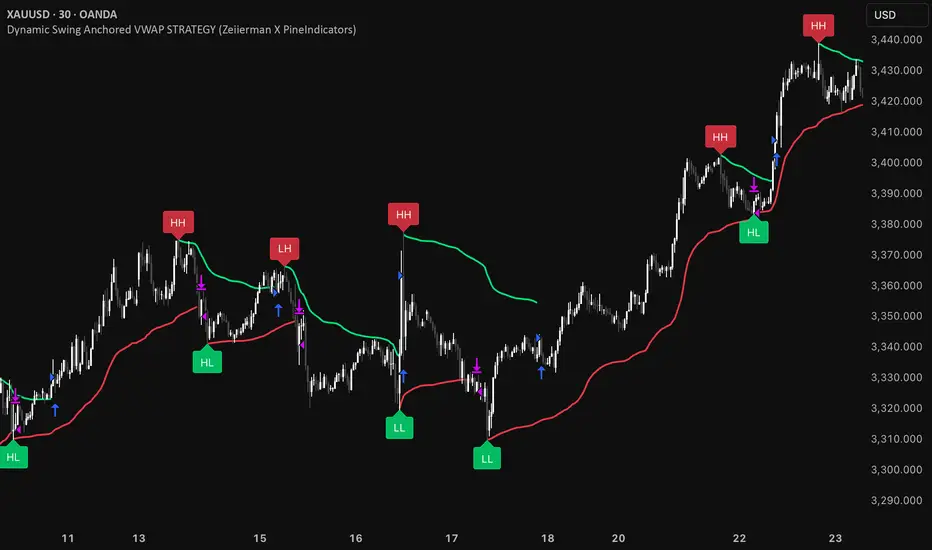
Long/Short/Exit/Risk management Strategy # LongShortExit Strategy Documentation
## Overview
The LongShortExit strategy is a versatile trading system for TradingView that provides complete control over entry, exit, and risk management parameters. It features a sophisticated framework for managing long and short positions with customizable profit targets, stop-loss mechanisms, partial profit-taking, and trailing stops. The strategy can be enhanced with continuous position signals for visual feedback on the current trading state.
## Key Features
### General Settings
- **Trading Direction**: Choose to trade long positions only, short positions only, or both.
- **Max Trades Per Day**: Limit the number of trades per day to prevent overtrading.
- **Bars Between Trades**: Enforce a minimum number of bars between consecutive trades.
### Session Management
- **Session Control**: Restrict trading to specific times of the day.
- **Time Zone**: Specify the time zone for session calculations.
- **Expiration**: Optionally set a date when the strategy should stop executing.
### Contract Settings
- **Contract Type**: Select from common futures contracts (MNQ, MES, NQ, ES) or custom values.
- **Point Value**: Define the dollar value per point movement.
- **Tick Size**: Set the minimum price movement for accurate calculations.
### Visual Signals
- **Continuous Position Signals**: Implement 0 to 1 visual signals to track position states.
- **Signal Plotting**: Customize color and appearance of position signals.
- **Clear Visual Feedback**: Instantly see when entry conditions are triggered.
### Risk Management
#### Stop Loss and Take Profit
- **Risk Type**: Choose between percentage-based, ATR-based, or points-based risk management.
- **Percentage Mode**: Set SL/TP as a percentage of entry price.
- **ATR Mode**: Set SL/TP as a multiple of the Average True Range.
- **Points Mode**: Set SL/TP as a fixed number of points from entry.
#### Advanced Exit Features
- **Break-Even**: Automatically move stop-loss to break-even after reaching specified profit threshold.
- **Trailing Stop**: Implement a trailing stop-loss that follows price movement at a defined distance.
- **Partial Profit Taking**: Take partial profits at predetermined price levels:
- Set first partial exit point and percentage of position to close
- Set second partial exit point and percentage of position to close
- **Time-Based Exit**: Automatically exit a position after a specified number of bars.
#### Win/Loss Streak Management
- **Streak Cutoff**: Automatically pause trading after a series of consecutive wins or losses.
- **Daily Reset**: Option to reset streak counters at the start of each day.
### Entry Conditions
- **Source and Value**: Define the exact price source and value that triggers entries.
- **Equals Condition**: Entry signals occur when the source exactly matches the specified value.
### Performance Analytics
- **Real-Time Stats**: Track important performance metrics like win rate, P&L, and largest wins/losses.
- **Visual Feedback**: On-chart markers for entries, exits, and important events.
### External Integration
- **Webhook Support**: Compatible with TradingView's webhook alerts for automated trading.
- **Cross-Platform**: Connect to external trading systems and notification platforms.
- **Custom Order Execution**: Implement advanced order flows through external services.
## How to Use
### Setup Instructions
1. Add the script to your TradingView chart.
2. Configure the general settings based on your trading preferences.
3. Set session trading hours if you only want to trade specific times.
4. Select your contract specifications or customize for your instrument.
5. Configure risk parameters:
- Choose your preferred risk management approach
- Set appropriate stop-loss and take-profit levels
- Enable advanced features like break-even, trailing stops, or partial profit taking as needed
6. Define entry conditions:
- Select the price source (such as close, open, high, or an indicator)
- Set the specific value that should trigger entries
### Entry Condition Examples
- **Example 1**: To enter when price closes exactly at a whole number:
- Long Source: close
- Long Value: 4200 (for instance, to enter when price closes exactly at 4200)
- **Example 2**: To enter when an indicator reaches a specific value:
- Long Source: ta.rsi(close, 14)
- Long Value: 30 (triggers when RSI equals exactly 30)
### Best Practices
1. **Always backtest thoroughly** before using in live trading.
2. **Start with conservative risk settings**:
- Small position sizes
- Reasonable stop-loss distances
- Limited trades per day
3. **Monitor and adjust**:
- Use the performance table to track results
- Adjust parameters based on how the strategy performs
4. **Consider market volatility**:
- Use ATR-based stops during volatile periods
- Use fixed points during stable markets
## Continuous Position Signals Implementation
The LongShortExit strategy can be enhanced with continuous position signals to provide visual feedback about the current position state. These signals can help you track when the strategy is in a long or short position.
### Adding Continuous Position Signals
Add the following code to implement continuous position signals (0 to 1):
```pine
// Continuous position signals (0 to 1)
var float longSignal = 0.0
var float shortSignal = 0.0
// Update position signals based on your indicator's conditions
longSignal := longCondition ? 1.0 : 0.0
shortSignal := shortCondition ? 1.0 : 0.0
// Plot continuous signals
plot(longSignal, title="Long Signal", color=#00FF00, linewidth=2, transp=0, style=plot.style_line)
plot(shortSignal, title="Short Signal", color=#FF0000, linewidth=2, transp=0, style=plot.style_line)
```
### Benefits of Continuous Position Signals
- Provides clear visual feedback of current position state (long/short)
- Signal values stay consistent (0 or 1) until condition changes
- Can be used for additional calculations or alert conditions
- Makes it easier to track when entry conditions are triggered
### Using with Custom Indicators
You can adapt the continuous position signals to work with any custom indicator by replacing the condition with your indicator's logic:
```pine
// Example with moving average crossover
longSignal := fastMA > slowMA ? 1.0 : 0.0
shortSignal := fastMA < slowMA ? 1.0 : 0.0
```
## Webhook Integration
The LongShortExit strategy is fully compatible with TradingView's webhook alerts, allowing you to connect your strategy to external trading platforms, brokers, or custom applications for automated trading execution.
### Setting Up Webhooks
1. Create an alert on your chart with the LongShortExit strategy
2. Enable the "Webhook URL" option in the alert dialog
3. Enter your webhook endpoint URL (from your broker or custom trading system)
4. Customize the alert message with relevant information using TradingView variables
### Webhook Message Format Example
```json
{
"strategy": "LongShortExit",
"action": "{{strategy.order.action}}",
"price": "{{strategy.order.price}}",
"quantity": "{{strategy.position_size}}",
"time": "{{time}}",
"ticker": "{{ticker}}",
"position_size": "{{strategy.position_size}}",
"position_value": "{{strategy.position_value}}",
"order_id": "{{strategy.order.id}}",
"order_comment": "{{strategy.order.comment}}"
}
```
### TradingView Alert Condition Examples
For effective webhook automation, set up these alert conditions:
#### Entry Alert
```
{{strategy.position_size}} != {{strategy.position_size}}
```
#### Exit Alert
```
{{strategy.position_size}} < {{strategy.position_size}} or {{strategy.position_size}} > {{strategy.position_size}}
```
#### Partial Take Profit Alert
```
strategy.order.comment contains "Partial TP"
```
### Benefits of Webhook Integration
- **Automated Trading**: Execute trades automatically through supported brokers
- **Cross-Platform**: Connect to custom trading bots and applications
- **Real-Time Notifications**: Receive trade signals on external platforms
- **Data Collection**: Log trade data for further analysis
- **Custom Order Management**: Implement advanced order types not available in TradingView
### Compatible External Applications
- Trading bots and algorithmic trading software
- Custom order execution systems
- Discord, Telegram, or Slack notification systems
- Trade journaling applications
- Risk management platforms
### Implementation Recommendations
- Test webhook delivery using a free service like webhook.site before connecting to your actual trading system
- Include authentication tokens or API keys in your webhook URL or payload when required by your external service
- Consider implementing confirmation mechanisms to verify trade execution
- Log all webhook activities for troubleshooting and performance tracking
## Strategy Customization Tips
### For Scalping
- Set smaller profit targets (1-3 points)
- Use tighter stop-losses
- Enable break-even feature after small profit
- Set higher max trades per day
### For Day Trading
- Use moderate profit targets
- Implement partial profit taking
- Enable trailing stops
- Set reasonable session trading hours
### For Swing Trading
- Use longer-term charts
- Set wider stops (ATR-based often works well)
- Use higher profit targets
- Disable daily streak reset
## Common Troubleshooting
### Low Win Rate
- Consider widening stop-losses
- Verify that entry conditions aren't triggering too frequently
- Check if the equals condition is too restrictive; consider small tolerances
### Missing Obvious Trades
- The equals condition is extremely precise. Price must exactly match the specified value.
- Consider using floating-point precision for more reliable triggers
### Frequent Stop-Outs
- Try ATR-based stops instead of fixed points
- Increase the stop-loss distance
- Enable break-even feature to protect profits
## Important Notes
- The exact equals condition is strict and may result in fewer trade signals compared to other conditions.
- For instruments with decimal prices, exact equality might be rare. Consider the precision of your value.
- Break-even and trailing stop calculations are based on points, not percentage.
- Partial take-profit levels are defined in points distance from entry.
- The continuous position signals (0 to 1) provide valuable visual feedback but don't affect the strategy's trading logic directly.
- When implementing continuous signals, ensure they're aligned with the actual entry conditions used by the strategy.
---
*This strategy is for educational and informational purposes only. Always test thoroughly before using with real funds.*

nineLivesUtilLibLibrary "nineLivesUtilLib"
isDateInRange(currentTime, useTimeFilter, startDate, endDate)
Checks if the current time is within the specified date range.
Parameters:
currentTime (int) : The current bar's time (time).
useTimeFilter (bool) : Bool 📅: Enable the date range filter.
startDate (int) : Timestamp 📅: The start date for the filter.
endDate (int) : Timestamp 📅: The end date for the filter.
Returns: True if the current time is within the range or filtering is disabled, false otherwise.
@example
inDateRange = nineLivesUtilLib.isDateInRange(time, useTimeFilter, startDate, endDate)
if inDateRange
// Execute trading logic
checkVolumeCondition(currentVolume, useVolumeFilter, volumeThresholdMultiplier, volumeLength)
Checks if the current volume meets the threshold condition.
Parameters:
currentVolume (float) : The current bar's volume (volume).
useVolumeFilter (bool) : Bool 📊: Enable the volume filter.
volumeThresholdMultiplier (float) : Float 📊: Volume threshold relative to average (e.g., 1.5 for 1.5x average).
volumeLength (int) : Int 📊: Lookback length for the volume average.
Returns: True if the volume condition is met or filtering is disabled, false otherwise.
@example
volumeOk = nineLivesUtilLib.checkVolumeCondition(volume, useVolumeFilter, volumeThreshold, volumeLength)
if volumeOk
// Proceed with trading logic
checkMultiTimeframeCondition(currentClose, currentOpen, htfClose, htfOpen, useMultiTimeframe, alignment)
Checks alignment with higher timeframe direction.
Parameters:
currentClose (float) : Float: The current bar's closing price (close).
currentOpen (float) : Float: The current bar's opening price (open).
htfClose (float) : Float: The closing price from the higher timeframe (must be fetched by the calling script using request.security).
htfOpen (float) : Float: The opening price from the higher timeframe (must be fetched by the calling script using request.security).
useMultiTimeframe (bool) : Bool ⏱️: Enable multi-timeframe analysis.
alignment (string) : String ⏱️: Desired alignment ("same", "opposite", "any").
Returns: True if the timeframe alignment condition is met or analysis is disabled, false otherwise.
@example
// In the calling script:
= request.security(syminfo.tickerid, higherTimeframe, )
tfOk = nineLivesUtilLib.checkMultiTimeframeCondition(close, open, htfClose, htfOpen, useMultiTimeframe, tfAlignment)
if tfOk
// Proceed with trading logic
checkMarketRegime(useMarketRegime, regimeIndicator, regimeThreshold, regimeLength, regimeMode)
Detects the market regime (trending or ranging) and checks if trading is allowed.
Parameters:
useMarketRegime (bool) : Bool 🔍: Enable market regime detection.
regimeIndicator (string) : String 🔍: Indicator to use ("ADX" or "Volatility").
regimeThreshold (int) : Int 🔍: Threshold for trend strength/volatility.
regimeLength (simple int) : Int 🔍: Lookback length for the indicator.
regimeMode (string) : String 🔍: Trading mode based on regime ("trend_only", "range_only", "adaptive").
Returns: A tuple containing:
: conditionMet (bool) - True if trading is allowed based on the regime mode and detection, false otherwise.
: inTrendingRegime (bool) - True if the current regime is trending based on the indicator and threshold.
@example
= nineLivesUtilLib.checkMarketRegime(useMarketRegime, regimeIndicator, regimeThreshold, regimeLength, regimeMode)
if regimeOk
// Proceed with trading logic
applyCooldown(buySignal, sellSignal, cooldownBars)
Applies a cooldown period after a signal.
Parameters:
buySignal (bool) : Bool: Buy signal (potentially after primary entry logic).
sellSignal (bool) : Bool: Sell signal (potentially after primary entry logic).
cooldownBars (int) : Int ⏳: The number of bars to wait after a signal before allowing another.
Returns: A tuple containing:
: cooldownFilteredBuy (bool) - Buy signal after cooldown filter.
: cooldownFilteredSell (bool) - Sell signal after cooldown filter.
@example
= nineLivesUtilLib.applyCooldown(rawBuySignal, rawSellSignal, iCool)
applyAllFilters(rawBuy, rawSell, inDateRange, tradeDirection, volumeOk, tfOk, regimeOk, drawdownOk, cooldownOkBuy, cooldownOkSell)
Applies all filtering conditions to the buy and sell signals.
Parameters:
rawBuy (bool) : Bool: The initial buy signal candidate (from primary entry logic, e.g., after cooldown).
rawSell (bool) : Bool: The initial sell signal candidate (from primary entry logic, e.g., after cooldown).
inDateRange (bool) : Bool 📅: Result from isDateInRange.
tradeDirection (string) : String 🔄: Overall trade direction preference ("longs_only", "shorts_only", "both").
volumeOk (bool) : Bool 📊: Result from checkVolumeCondition.
tfOk (bool) : Bool ⏱️: Result from checkMultiTimeframeCondition.
regimeOk (bool) : Bool 🔍: Result from checkMarketRegime.
drawdownOk (bool) : Bool 📉: Result from checkDrawdownExceeded (or equivalent).
cooldownOkBuy (bool) : Bool ⏳: Result from applyCooldown for buy.
cooldownOkSell (bool) : Bool ⏳: Result from applyCooldown for sell.
Returns: A tuple containing:
: finalBuySignal (bool) - The final buy signal after all filters.
: finalSellSignal (bool) - The final sell signal after all filters.
@example
= nineLivesUtilLib.applyAllFilters(cooldownBuy, cooldownSell, inDateRange, tradeDirection, volumeOk, tfOk, regimeOk, !drawdownExceeded, cooldownBuy, cooldownSell)
NOTE: This function filters signals generated by your primary entry logic (e.g., EMA crossover).
checkDrawdownExceeded(currentEquity, useMaxDrawdown, maxDrawdownPercent)
Tracks maximum equity and checks if current drawdown exceeds a threshold.
Parameters:
currentEquity (float) : Float: The strategy's current equity (strategy.equity).
useMaxDrawdown (bool) : Bool 📉: Enable max drawdown protection.
maxDrawdownPercent (float) : Float 📉: The maximum allowed drawdown as a percentage.
Returns: True if drawdown protection is enabled and the current drawdown exceeds the threshold, false otherwise.
@example
drawdownExceeded = nineLivesUtilLib.checkDrawdownExceeded(strategy.equity, useMaxDrawdown, maxDrawdownPercent)
if drawdownExceeded
// Consider stopping entries or exiting positions in the strategy script
calculateExitPrice(positionAvgPrice, percentage, isStop, isLong)
Calculates a stop loss or take profit price based on a percentage from the average entry price.
Parameters:
positionAvgPrice (float) : Float: The average price of the current position (strategy.position_avg_price).
percentage (float) : Float: The stop loss or take profit percentage (e.g., 2.0 for 2%).
isStop (bool) : Bool: True if calculating a stop loss price, false if calculating a take profit price.
isLong (bool) : Bool: True if the position is long, false if short.
Returns: The calculated stop price or take profit price, or na if no position or percentage is invalid.
@example
longSL = nineLivesUtilLib.calculateExitPrice(strategy.position_avg_price, stopLossPercent, true, true)
shortTP = nineLivesUtilLib.calculateExitPrice(strategy.position_avg_price, takeProfitPercent, false, false)
calculateTrailingStopLevel(positionAvgPrice, trailOffsetPercent, trailPercent, currentHigh, currentLow, isLong)
Calculates the current trailing stop level for a position.
Parameters:
positionAvgPrice (float) : Float: The average price of the current position (strategy.position_avg_price).
trailOffsetPercent (float) : Float 🔄: The percentage price movement to activate the trailing stop.
trailPercent (float) : Float 🔄: The percentage distance the stop trails behind the price.
currentHigh (float) : Float: The current bar's high (high).
currentLow (float) : Float: The current bar's low (low).
isLong (bool) : Bool: True if the position is long, false if short.
Returns: The calculated trailing stop price if active, otherwise na.
@example
longTrailStop = nineLivesUtilLib.calculateTrailingStopLevel(strategy.position_avg_price, trailOffset, trailPercent, high, low, true)
shortTrailStop = nineLivesUtilLib.calculateTrailingStopLevel(strategy.position_avg_price, trailOffset, trailPercent, high, low, false)
if not na(longTrailStop)
strategy.exit("Long Trail", from_entry="Long", stop=longTrailStop)